00 Overview
Class 5 — lecture of 12 Sep 2026, eleven scanned pages (six of theory, five of solved problems) — stays at the electrode/electrolyte interface and goes one level deeper. Class 4 ended with : current as rate. But an electrode at equilibrium passes zero net current while both half-reactions keep running at equal rates. That hidden equal-and-opposite current is the exchange current , and it sets the scale of all electrode kinetics. Push the potential away from equilibrium by the overpotential and the two rates unbalance — the current–overpotential curve is the Butler–Volmer equation, whose high-overpotential shadow is the Tafel equation .
— exchange current density: how fast electron transfer can run at equilibrium (Sections 2–3). — overpotential: the drive away from equilibrium, signed anodic/cathodic (Section 4). Butler–Volmer — the full current–overpotential law, two exponentials (Sections 5–6). Tafel — its straight-line high- limit, the working tool of electrochemistry (Sections 8–11).
- Sections 1–3 build from the two partial currents and the dynamic-equilibrium picture.
- Sections 4–5 define , its sign convention, and why a barrier change moves the current.
- Section 6 + lab 12 state the Butler–Volmer equation and let you drag , , , across it.
- Sections 7–11 + lab 13 derive the three regimes, both Tafel equations, the slopes , and how a Tafel plot hands back .
- Sections 12–14 the memory chain, then the lecture's own twelve solved problems, worked in full.
- Sections 15–20 calculator, equation sheet, symbol table, rapid revision, raw scans, PYQ audit.
01 Two reactions, two partial currents
Starting with a general electrode reaction,
At the electrode surface, two opposite reactions can occur at the same time:
- Reduction: — carrying the cathodic current ;
- Oxidation: — carrying the anodic current .
Therefore there are two partial currents, and what an ammeter reads is their difference — boxed on the first scanned page:
02 Exchange current & exchange current density ()
Suppose the electrode is at equilibrium. Then
But this does not mean the reactions have stopped — both are still occurring, at equal rates. The current corresponding to either reaction at equilibrium is called the exchange current, ; expressed per unit area,
and this is called the exchange current density.
The equilibrium of an electrode is a dynamic equilibrium in exactly the same sense as a chemical equilibrium: forward and backward rates equal, neither zero. is the magnitude of each of the two hidden currents — the pulse of the interface at rest.
03 What tells you — physical meaning
Exchange current density tells us how rapidly electron transfer can occur at an electrode under equilibrium conditions. The notebook's two-line reading:
- Large → fast electrode kinetics (the interface swaps electrons readily — e.g. Pt/H₂-type electrodes);
- Small → slow electrode kinetics (the interface is sluggish; even a tiny net current needs a real push).
is a property of the pair (electrode material + redox couple + solution), not of the couple alone: the same Fe³⁺/Fe²⁺ reaction runs at different on different metals. That is why tables of are tables of electrode kinetics itself.
04 What happens when we apply a potential — overpotential
Now suppose we move the electrode potential away from its equilibrium value. The electrode potential required by equilibrium is called . If the actual electrode potential is , then the difference is called overpotential or overvoltage — boxed:
Sign of overpotential
- If the electrode is driven in the oxidation direction: and the anodic current becomes dominant;
- If the electrode is driven in the reduction direction: and the cathodic current becomes dominant.
So: anodic process; cathodic process.
05 Why does the current change?
When an overpotential is applied, the energy barrier for electron transfer changes. Therefore the rates of oxidation and reduction change. Since
the current also changes. This relationship between current and overpotential is described by the Butler–Volmer equation.
Class 4 taught — current proportional to rate. Class 5 adds the missing link: tilts the activation barrier, the barrier tilts the rates, the rates tilt the two partial currents, and their difference is the measured current. One chain: barrier rates .
06 The Butler–Volmer equation
The general Butler–Volmer equation is
where
- = net current density; = exchange current density;
- = number of electrons transferred; = Faraday constant;
- = gas constant; = absolute temperature;
- = overpotential; = charge-transfer coefficient, usually .
Butler–Volmer without mathematics
The equation contains two terms — anodic term − cathodic term, i.e. . Therefore the Butler–Volmer equation essentially says:
“The net current is the difference between the anodic and cathodic currents, and both currents depend exponentially on overpotential.” This is the main idea.
Butler–Volmer, live
Drag the overpotential along the curve and watch the two exponentials unbalance. The vertical scale is symlog (asinh of i in units of i(0)) so the straight linear region near η = 0 and the explosive Tafel tails share one frame; the readouts below quote the exact currents in A cm⁻².
Illustrates Section 6 (and the three regimes of Section 7): the curve is i = i(0)[e^(αnFη/RT) − e^(−(1−α)nFη/RT)] at T = 298 K, evaluated exactly; at η = 0 the readouts return i = 0 with i(a) = i(c) = i(0), the dynamic equilibrium of Section 2. Vertical axis is symlog for visibility only — never use it to read magnitudes; the readouts are the physics. Fully static under reduced motion (no animation involved).
07 Three regimes of — one equation, three faces
At equilibrium ()
Putting in the Butler–Volmer equation: , but . So, exchange current density is present even though the net current is zero.
At small overpotential
When is very small the equation can be simplified using for small :
This region is called the linear or low-overpotential region.
At high overpotential
When the overpotential becomes sufficiently large, one of the two terms becomes much larger than the other — and the equation collapses to a single exponential on each side (Sections 8–9).
08 Large positive — the anodic Tafel equation
At large positive overpotential the anodic current dominates:
Taking natural logarithms on both sides, , or — boxed in the notebook —
This is the anodic Tafel equation.
09 Large negative — the cathodic Tafel equation
At sufficiently large negative overpotential the cathodic term dominates:
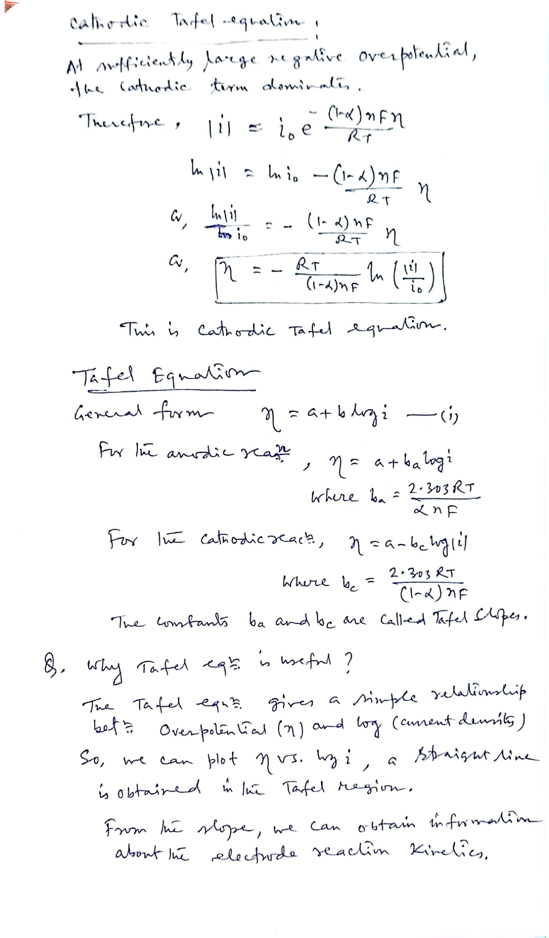
so , i.e. — boxed —
This is the cathodic Tafel equation.
10 The Tafel equation and the Tafel slopes
Both limits wear one common costume — the general form, with = log₁₀:
- Anodic reaction: , where
- Cathodic reaction: , where
The constants and are called the Tafel slopes. (The 2.303 is just : converting natural logs to decades.)
The Tafel equation gives a simple relationship between overpotential and log(current density): plot vs and a straight line appears in the Tafel region. From its slope and intercept we obtain information about the electrode reaction kinetics — , and itself (Section 11).
11 Reading a Tafel plot — how to determine
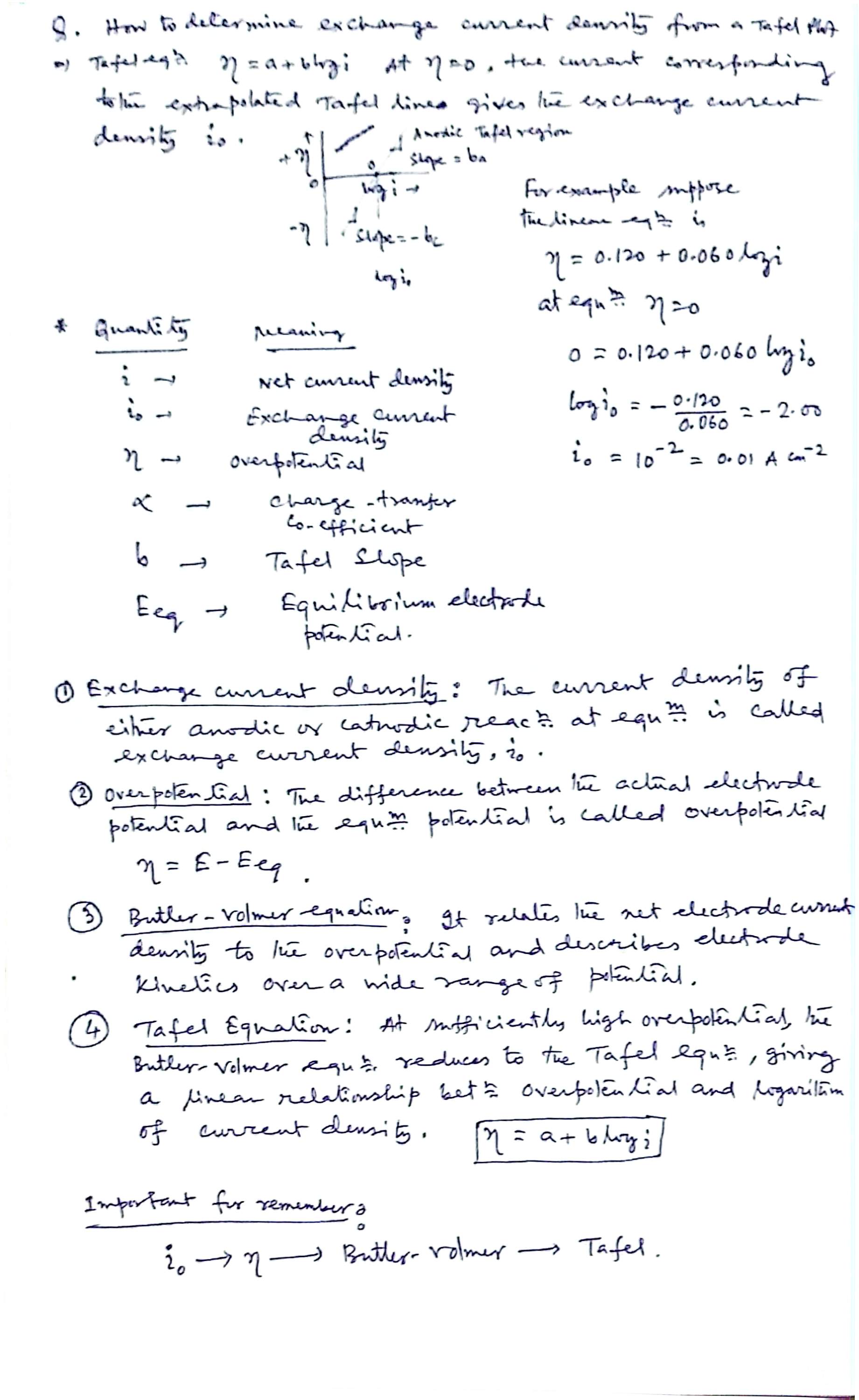
From the Tafel equation : at , the current corresponding to the extrapolated Tafel line gives the exchange current density . The notebook's sketch shows both branches — anodic Tafel region with slope above, cathodic with slope below — meeting the axis at .
Q. Suppose the linear (anodic Tafel) equation is . Find .
Ans. At equilibrium : $0 = 0.120 + 0.060 \log i_0 \Rightarrow \log i_0 = -0.120/0.060 = -2.00 \Rightarrow i_0 = 10^{-2} = 0.01$ A cm⁻².
Build a Tafel plot, read i(0) back
Two straight lines, one intersection: the anodic and cathodic Tafel branches both pass through (log i(0), 0). Slide the slope and the intercept and watch the whole plot rebuild — then read the exchange current density straight off the η = 0 crossing, exactly as the notebook's extrapolation does.
Illustrates Sections 10–11: η = a + b log i with a = −b log i(0); the anodic branch rises with slope +b, the cathodic mirror with −b, and both cross η = 0 at log i(0) — the extrapolation the notebook uses to extract i(0) from a measured plot. Try b = 0.060, log i(0) = −2 to reproduce the lecture's worked line η = 0.120 + 0.060 log i. Static by construction; reduced motion changes nothing because nothing animates.
12 The chain and the quantities
| Quantity | Meaning (notebook table) |
|---|---|
| net current density | |
| exchange current density | |
| overpotential | |
| charge-transfer coefficient | |
| Tafel slope | |
| equilibrium electrode potential |
(1) Exchange current density: the current density of either anodic or cathodic reaction at equilibrium is called exchange current density, . (2) Overpotential: the difference between the actual electrode potential and the equilibrium potential, . (3) Butler–Volmer equation: relates the net electrode current density to the overpotential and describes electrode kinetics over a wide range of potential. (4) Tafel equation: at sufficiently high overpotential the Butler–Volmer equation reduces to the Tafel equation, giving a linear relationship between overpotential and the logarithm of current density, .
Important for remembering: Butler–Volmer Tafel.
13 The lecture's solved problems I (1–6)
The second scan booklet is a pure problem set — twelve worked numericals under the heading “Butler–Volmer eqⁿ, exchange current density, overpotential, Tafel equation”. Reproduced in full, arithmetic checked.
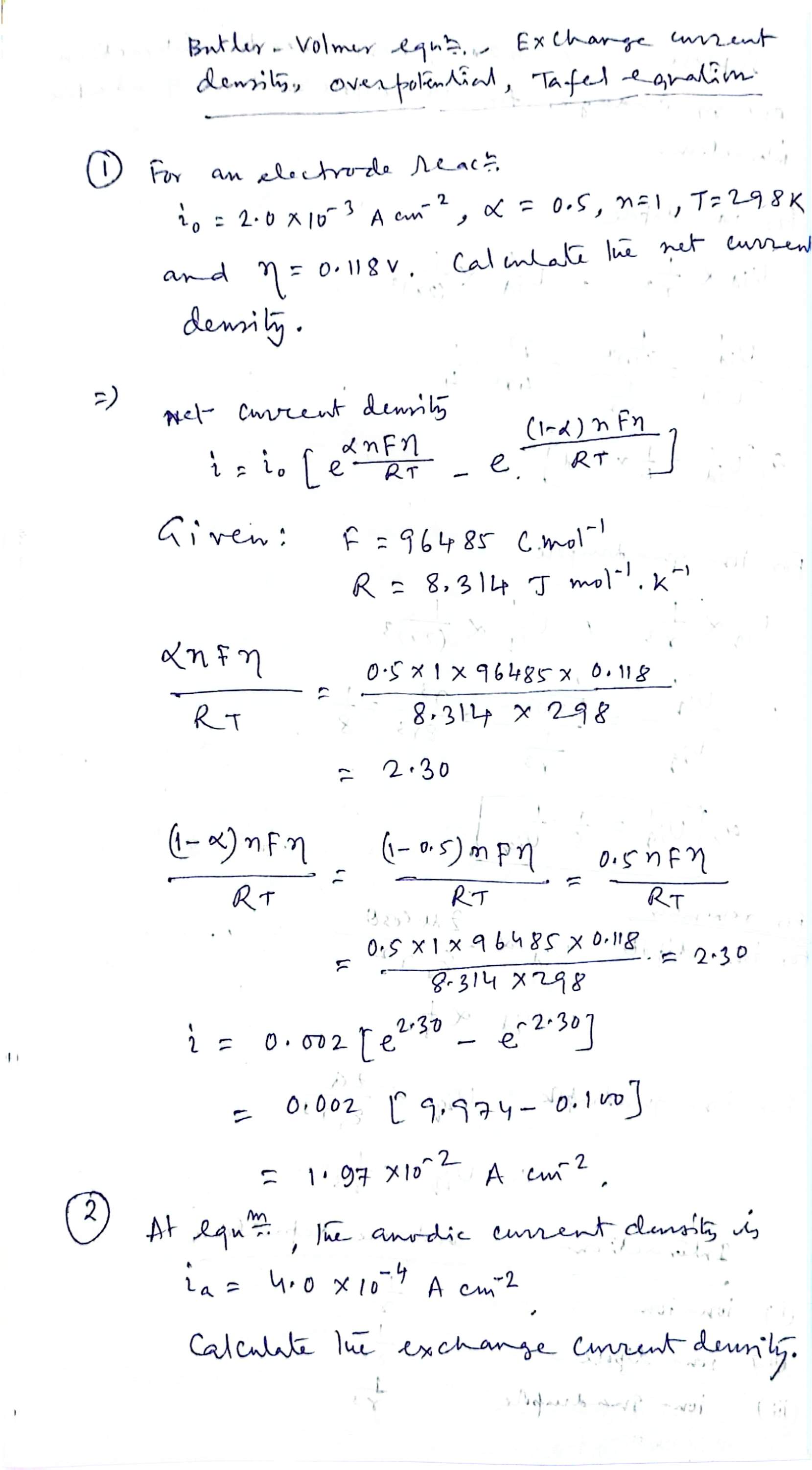
Q. For an electrode reaction A cm⁻², , , K and V. Calculate the net current density.
Ans. . With C mol⁻¹, J mol⁻¹ K⁻¹: , and with the cathodic exponent has the same magnitude: . .
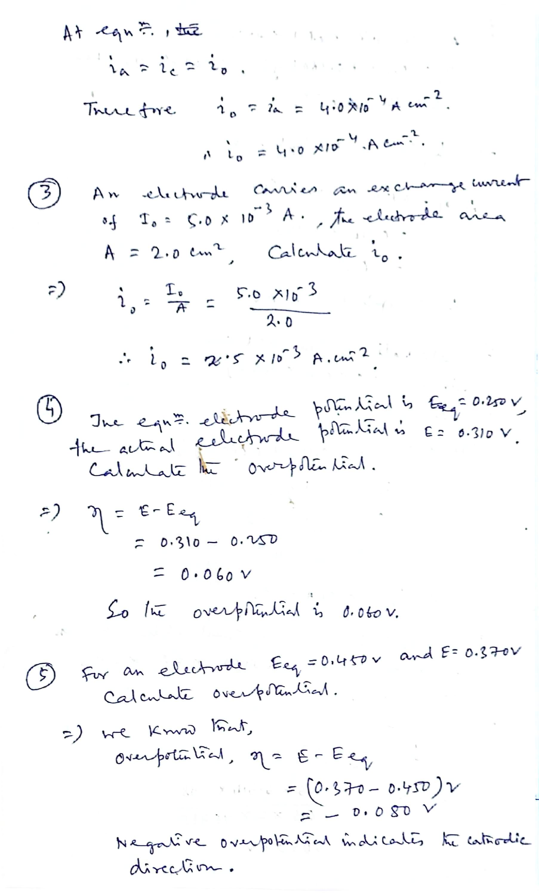
Q. At equilibrium the anodic current density is A cm⁻². Calculate the exchange current density.
Ans. At equilibrium , therefore .
Q. An electrode carries an exchange current of A; the electrode area is cm². Calculate .
Ans. .
Q. The equilibrium electrode potential is V; the actual electrode potential is V. Calculate the overpotential.
Ans. — positive, so the anodic direction is driven.
Q. For an electrode V and V. Calculate the overpotential.
Ans. . Negative overpotential indicates the cathodic direction.
Q. An anodic Tafel equation is . Calculate when A cm⁻².
Ans. , so — that current is the exchange current, so the drive needed is zero.
14 The lecture's solved problems II (7–12)
Q. Calculate from the Tafel equation, given .
Ans. At equilibrium : .
Q. Calculate the anodic Tafel slope for an electrode reaction involving , at 298 K.
Ans. (per decade).
Q. Calculate the overpotential from the Tafel equation, given A cm⁻², V decade⁻¹ and A cm⁻².
Ans. .
Q. Calculate the current from the Tafel equation, given V, A cm⁻², V decade⁻¹.
Ans. .
Q. Find from a Tafel plot intercept: the extrapolated x-intercept of vs is .
Ans. .
Q. Two points from the linear Tafel region are and . Calculate the Tafel slope.
Ans. .
15 Play with Butler–Volmer & Tafel
The whole lecture in one panel: set the exchange current density, charge-transfer coefficient, electron count, temperature and overpotential — the panel returns both partial currents, the exact Butler–Volmer net current, the linear-region approximation and the two Tafel slopes.
Checks against the lecture: Prob. 1 (i(0) = 2 × 10⁻³, α = 0.5, n = 1, 298 K, η = 0.118 V) → exponents ±2.30, i = 0.002(9.974 − 0.100) = 1.97 × 10⁻² A cm⁻²; at η = 0 the net reads exactly 0 while both branches read i(0); with n = 2, α = 0.5, 298 K the anodic slope reads 0.0591 V/decade (Prob. 8). The linear column only agrees with the exact one while |η| is small — that disagreement is precisely the Tafel region appearing.
16 The equation sheet, at a glance
Every boxed result of the lecture on one screen; labels match the sections above.
17 Symbol table
| Symbol | Meaning | Typical unit |
|---|---|---|
| Net current density (anodic minus cathodic) | A cm⁻² | |
| Anodic / cathodic partial current density | A cm⁻² | |
| Exchange current (whole electrode) | A | |
| Exchange current density, — either partial current at equilibrium | A cm⁻² | |
| Electrode area | cm² | |
| Actual electrode potential; equilibrium electrode potential | V | |
| Overpotential (overvoltage), ; >0 anodic, <0 cathodic | V | |
| Charge-transfer coefficient, usually | dimensionless | |
| Electrons transferred in the electrode reaction | dimensionless | |
| Faraday constant | 96 485 C mol⁻¹ | |
| Gas constant | 8.314 J mol⁻¹ K⁻¹ | |
| Absolute temperature | K | |
| Tafel intercept constant; Tafel slope ( anodic, cathodic) | V; V decade⁻¹ | |
| Ox, Red | Oxidised / reduced species of the general reaction | — |
18 Rapid revision — 14 lines before the exam
- General reaction (e.g. Fe³⁺ + e⁻ ⇌ Fe²⁺); both directions run at once at the surface.
- Partial currents: cathodic, anodic; boxed net .
- At equilibrium so — but neither reaction stops; either one's current = exchange current.
- = exchange current density; large → fast kinetics, small → slow kinetics.
- Overpotential ; anodic-dominant, cathodic-dominant.
- Why current changes: η changes the electron-transfer barrier → rates change → current changes (current ∝ rate).
- Butler–Volmer: ; anodic term minus cathodic term, both exponential in η.
- η = 0 ⇒ i = 0 but : exchange current density exists with zero net current.
- Small η: ⇒ — the linear (low-overpotential) region.
- High +η: anodic Tafel ; high −η: cathodic Tafel .
- General Tafel ; slopes , (V per decade).
- Tafel plot η vs log i: straight in the Tafel region; extrapolate to η = 0 to read (example: 0.120 + 0.060 log i ⇒ i₀ = 0.01 A cm⁻²).
- Slope from two points: (Prob. 12: 0.12/2 = 0.060 V decade⁻¹); at 298 K, n=2, α=0.5 ⇒ b(a) ≈ 0.0591 V.
- Memory chain: Butler–Volmer Tafel.
19 Original notebook scans
Digitised from the class notebook of 12 Sep 2026 — two CamScanner booklets: six theory pages (S1–S6, scanned 19:26) and five solved-problem pages (S7–S11, scanned 21:47). Every equation above was cross-checked against these pages, and every numerical re-computed. Tap any thumbnail to open the full scan.
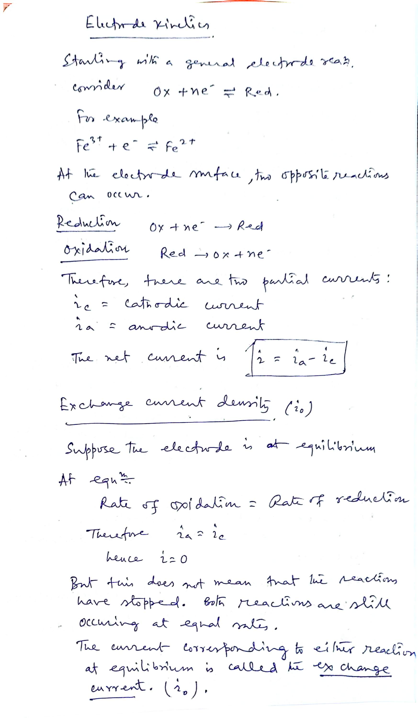 S1 · partial currents, boxed i = i(a) − i(c), exchange current
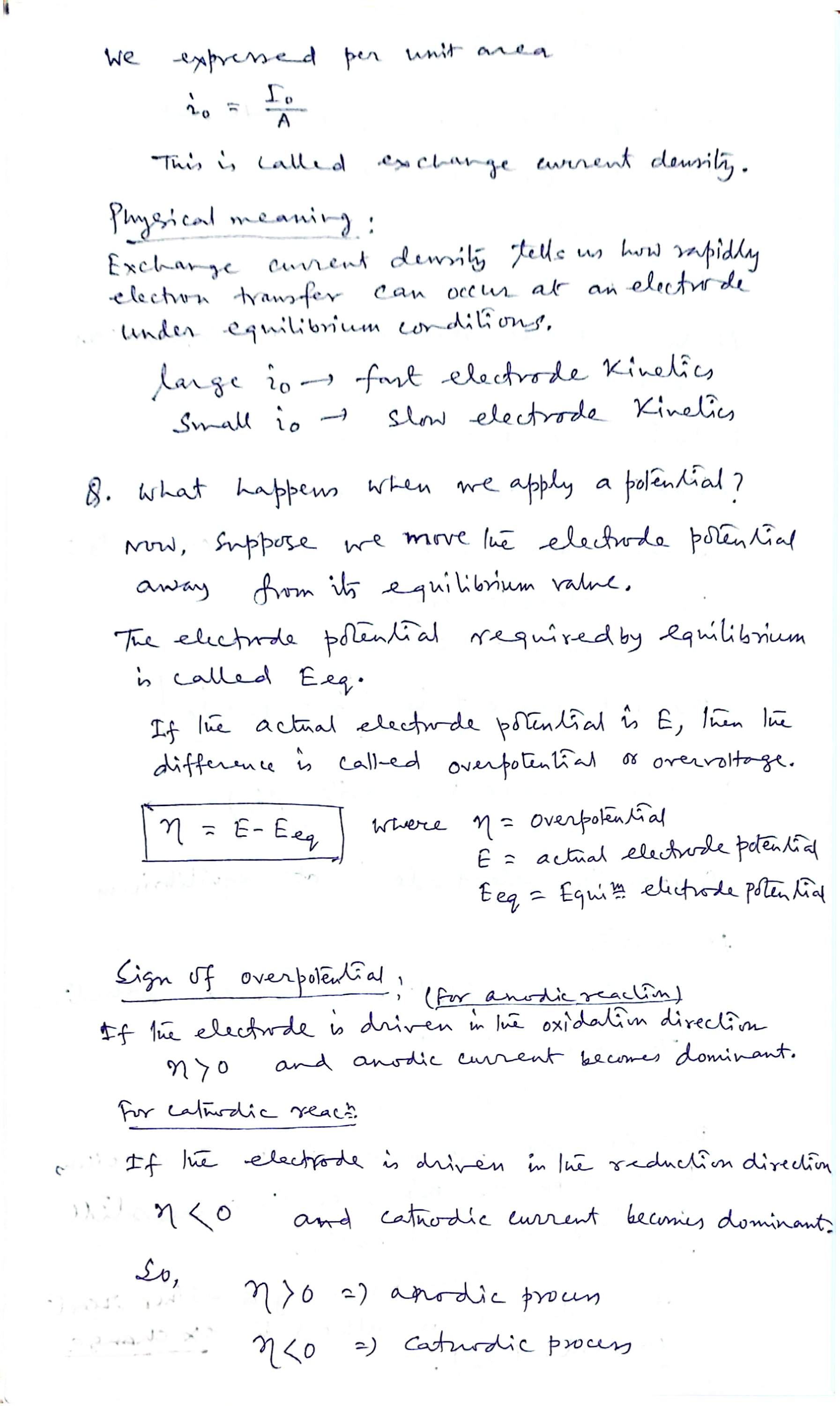 S2 · i(0) = I(0)/A, meaning, η = E − E(eq) + signs
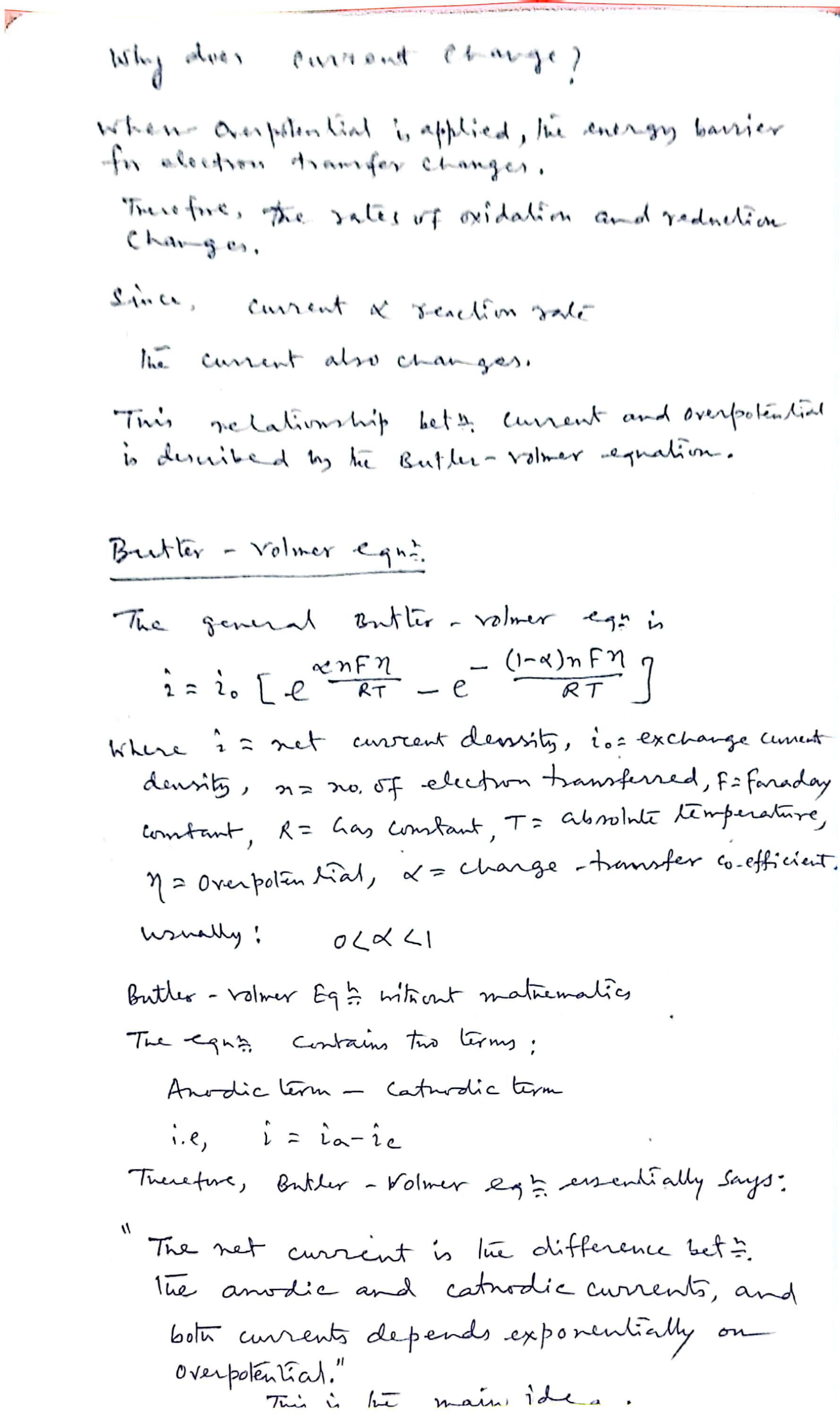 S3 · why current changes, Butler–Volmer equation, 0 < α < 1
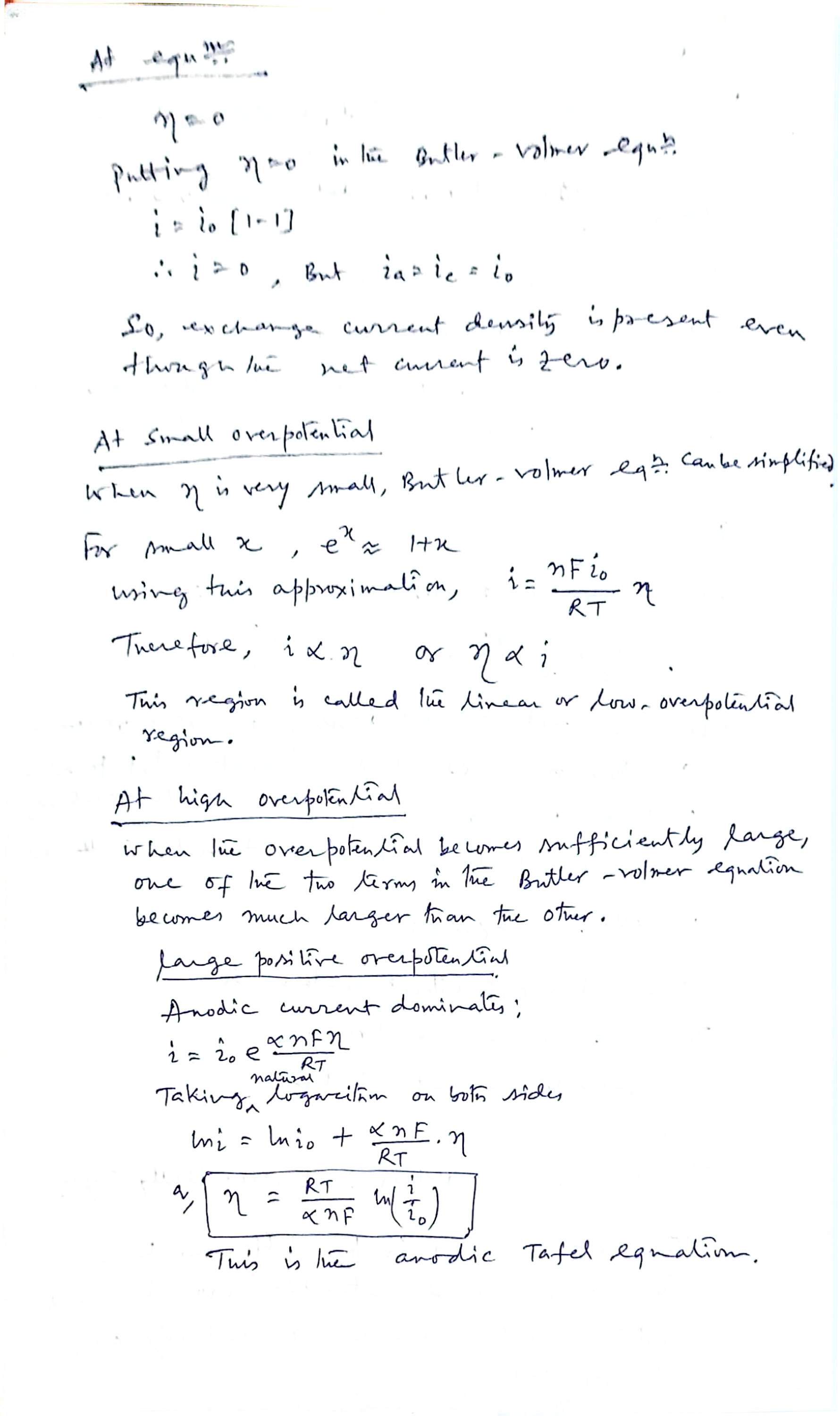 S4 · η = 0 check, linear region, anodic Tafel boxed
 S5 · cathodic Tafel boxed, general Tafel, slopes, why useful
 S6 · i(0) from Tafel plot + example, quantity table, 4-point summary
 S7 · Prob 1 (B–V net current), Prob 2 start
 S8 · Prob 2–5 (i(0), density, two overpotentials)
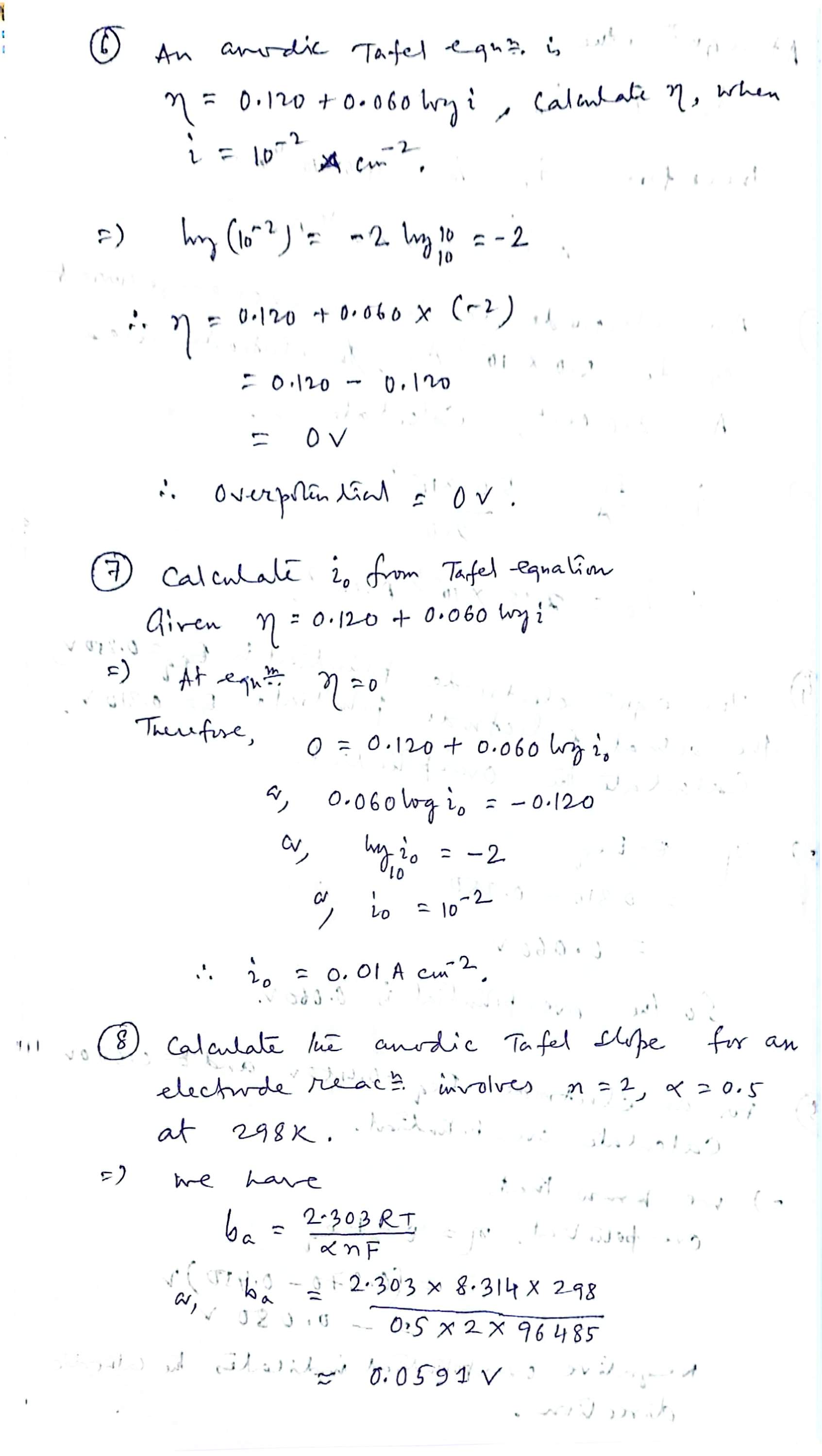 S9 · Prob 6–8 (η from Tafel, i(0), slope b(a))
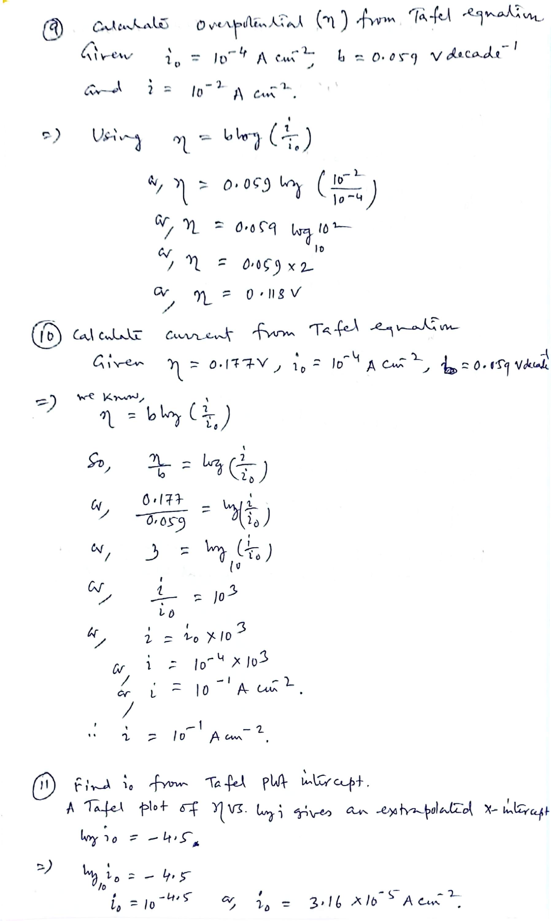 S10 · Prob 9–11 (η, i, plot intercept)
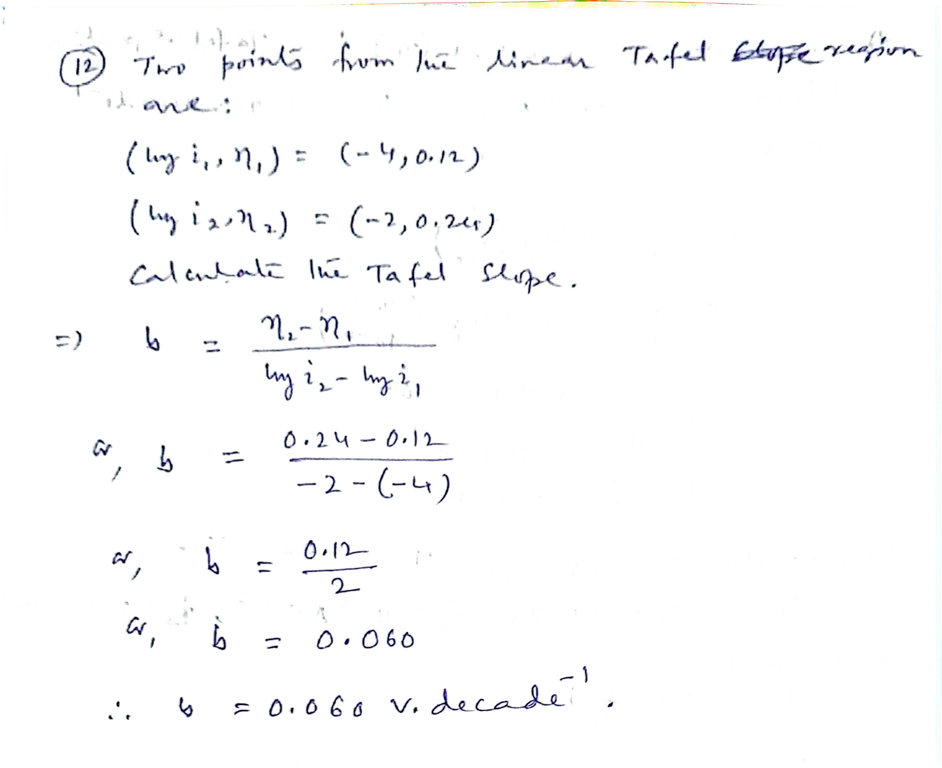 S11 · Prob 12 (two-point Tafel slope)
20 PYQ bank · University papers 2020–2024
Same audit as Classes 1–4: every page of the five M.Sc. Semester-I question papers (2020–2024 — all subjects MSCH-101…106, 60 scanned pages) OCR'd and verified by hand; the Physical Chemistry paper each year is MSCH-104 (Physical General-I). The rule is unchanged: only questions that actually appeared, tagged with year and repeat count.
| Year | Physical paper (MSCH-104) | Pages verified | Class-5 questions (exchange current / overpotential / Butler–Volmer / Tafel) |
|---|---|---|---|
| 2020 | Physical General I (new + old syllabus copies) | p. 12–15 | 0 — group theory, QM, stat-thermo, rotational/vibrational spectroscopy, fullerenes |
| 2021 | Physical General I (+ internal) | p. 7–8 | 0 — group theory, QM, partition functions, nanotubes, Raman |
| 2022 | Physical General I | p. 9–10 | 0 — symmetry, operators, spectroscopy, stat-thermo |
| 2023 | Physical General I | p. 9–10 | 0 — point groups, operators, rotors, Raman, fullerenes, stat-thermo |
| 2024 | Physical General I | p. 12–13 | 0 — group theory, matrices, rotors, polarizability, partition functions |
A fresh keyword sweep for this lecture's vocabulary (tafel | butler | volmer | overpotential | overvoltage | exchange current) across all 60 OCR'd pages returns zero hits — MSCH-104 in 2020–2024 never touched electrode kinetics — so, per the rule, the year-tagged bank stays empty rather than being padded with look-alikes. The moment one appears it lands here with its year and repeat count. For practice, the lecture itself supplied twelve fully solved problems: they are reproduced in Sections 13–14, which is the best problem set this topic could ask for.