Class 02 · Solvation Number & the Eley–Evans Model

00 Overview

Class 1 ended with the Born model: the whole solvent as one continuous dielectric. Class 2 — notebook pages 10–26, lecture of 22 Aug 2026 — asks the next question: how many solvent molecules are actually glued to the ion? That number, the solvation number $n$ , is the thread that ties the entire lecture together, and it is attacked from two sides.

Two answers to one question

Theory (Sections 4–7): the Eley–Evans model splits solvation into a discrete ion–dipole inner shell and a Born-type outer continuum. Experiment (Sections 8–10): three independent routes to $n$ — density / apparent molar volume, viscosity / Jones–Dole, and conductance / ionic mobility — each ending in its own boxed working formula.

Sections 1–3 define $n$ , the primary / secondary shells, the five factors that change it, and why it is only ever an average.
Sections 4–7 derive the Eley–Evans equation step by step and put it side-by-side with Born.
Sections 8–10 turn $n$ into a measurable quantity (density → viscosity → conductance).
Sections 11–16 live calculator, equation sheet, symbol table, rapid revision, the raw scans, and the PYQ audit 2020–24.

01 Solvation number & the two solvation shells

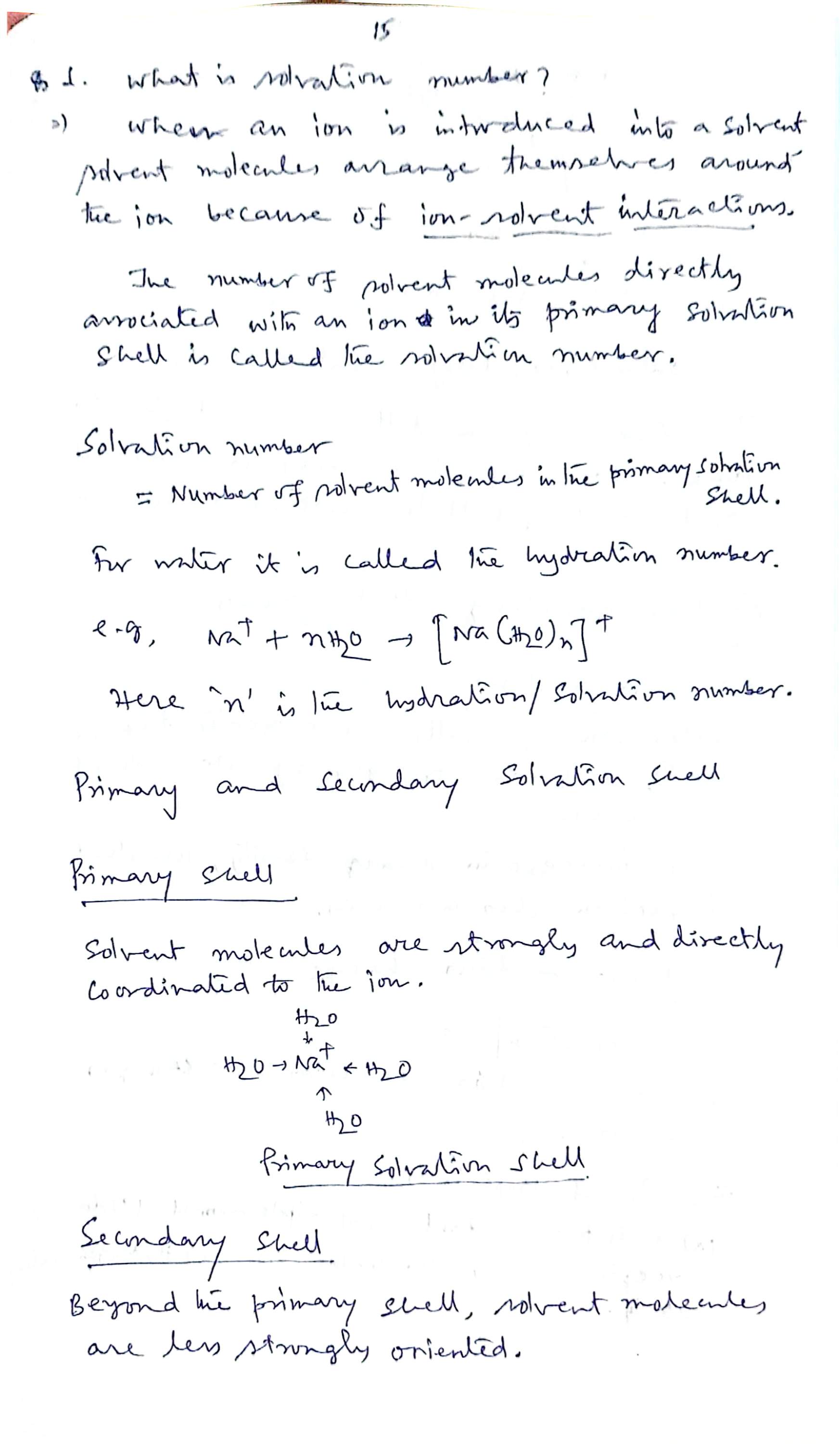
When an ion is introduced into a solvent, solvent molecules arrange themselves around the ion because of ion–solvent interactions. The number of solvent molecules directly associated with an ion in its primary solvation shell is called the solvation number:

def

Solvation number = number of solvent molecules in the primary solvation shell

For water as the solvent the same quantity is called the hydration number. The lecture's example:

\mathrm{Na}^{+} + n\,\mathrm{H_2O} \longrightarrow \left[\mathrm{Na(H_2O)}_{n}\right]^{+}

and, for a general solvent S around an ion M $^{z+}$ :

\mathrm{M}^{z+} + n\,\mathrm{S} \rightleftharpoons \left[\mathrm{M(S)}_{n}\right]^{z+}

Here $n$ is the hydration / solvation number.

Primary vs secondary shell

Primary shell: solvent molecules are strongly and directly coordinated to the ion (for Na⁺ in water the O ends point inward).
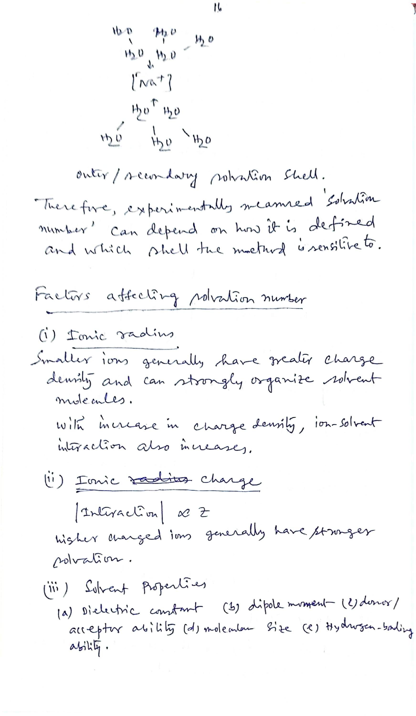
Secondary (outer) shell: beyond the primary shell, solvent molecules are less strongly oriented — perturbed, but never locked in.

Why the definition matters

Because a secondary shell exists, the experimentally measured “solvation number” can depend on how it is defined and on which shell the method is sensitive to. Carry this sentence into Sections 8–10: three methods, three slightly different numbers — all of them “the” solvation number.

02 What changes the solvation number

Five factors, exactly as listed in the notebook.

(i) Ionic radius

Smaller ions generally have greater charge density and can strongly organise solvent molecules; with an increase in charge density the ion–solvent interaction also increases.

(ii) Ionic charge

$\lvert \text{interaction} \rvert \propto z$ — higher-charged ions generally have stronger solvation.

(iii) Solvent properties

(a) dielectric constant
(b) dipole moment
(c) donor / acceptor ability
(d) molecular size
(e) hydrogen-bonding ability

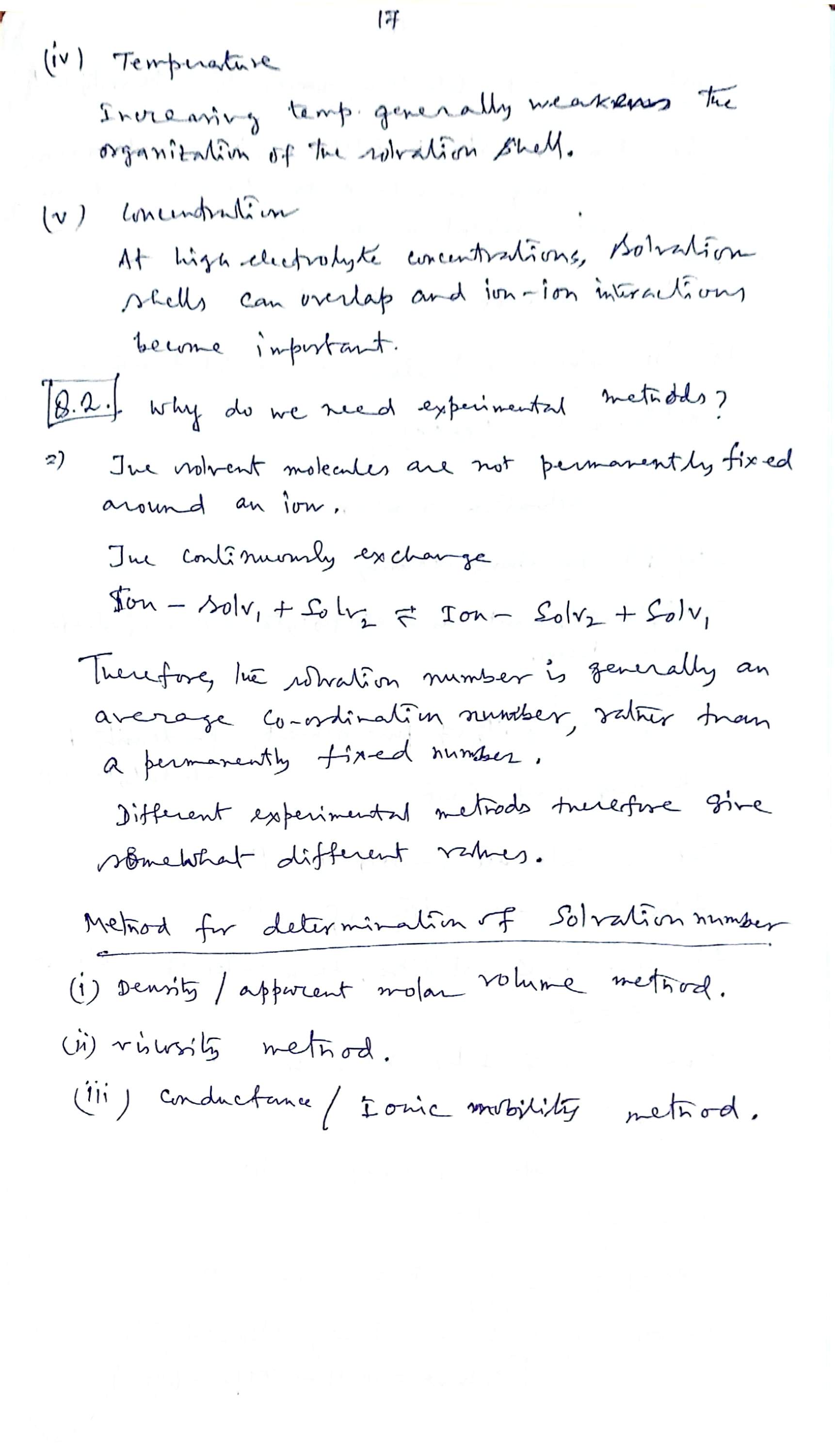
(iv) Temperature

Increasing temperature generally weakens the organisation of the solvation shell.

(v) Concentration

At high electrolyte concentrations the solvation shells can overlap and ion–ion interactions become important.

03 Why n must be measured: solvent exchange

Solvent molecules are not permanently fixed around an ion — they continuously exchange:

iii

\text{Ion–Solv}_1 + \text{Solv}_2 \rightleftharpoons \text{Ion–Solv}_2 + \text{Solv}_1

Therefore the solvation number is generally an average coordination number, rather than a permanently fixed number — and different experimental methods therefore give somewhat different values. The lecture lists three routes:

Density / apparent molar volume method (Section 8)
Viscosity method (Section 9)
Conductance / ionic mobility method (Section 10)

visual lab 3

The shell breathes: primary, secondary, bulk — and exchange

Inner ring = primary shell (oriented, O ends in). Middle ring = secondary shell (half-committed, wobbling). Scatter = bulk. Every few seconds a primary molecule trades places with a bulk one — the exchange equilibrium of Section 3, live.

Primary shell n

exchanges witnessed: 0 primary occupancy: time-averaged, not fixed

Because bound molecules keep swapping, every experimental n (Sections 8–10) is an average coordination number, and methods that sense different shells return slightly different values — the whole point of Section 3.

04 The Eley–Evans model: discrete solvent where it matters

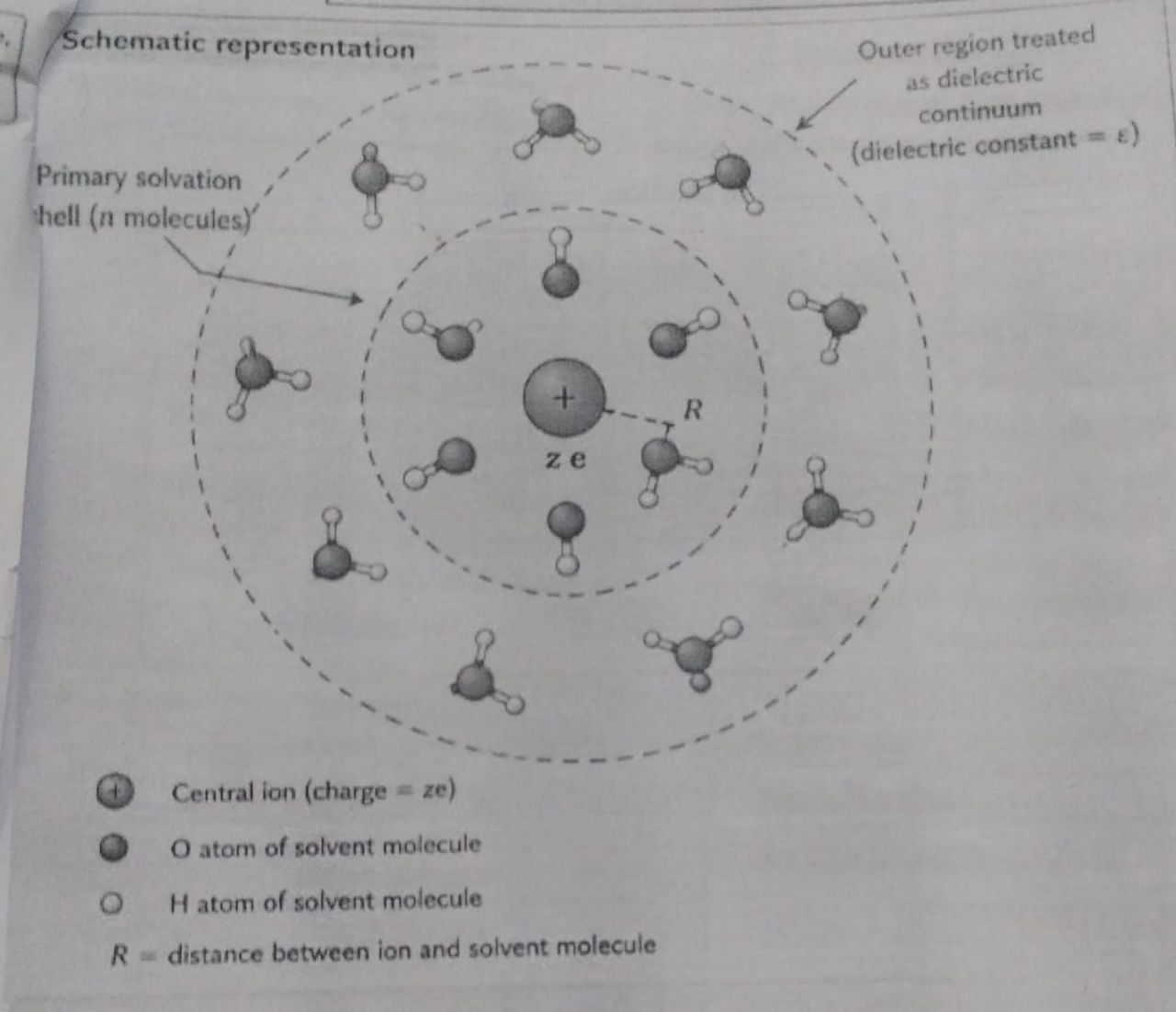
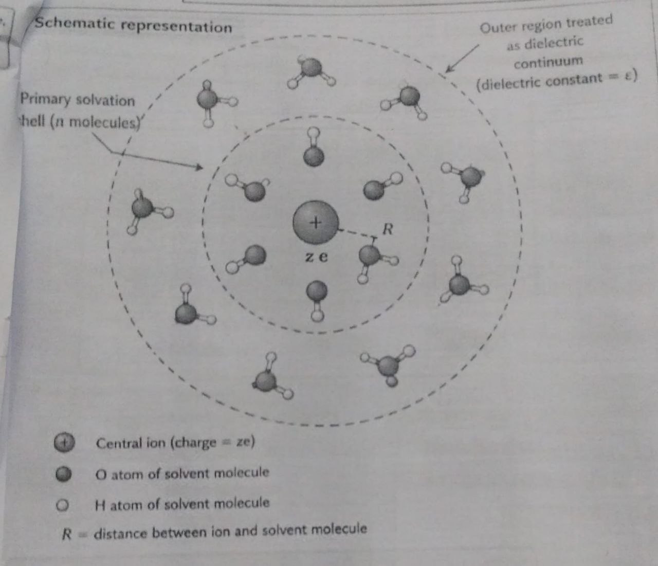
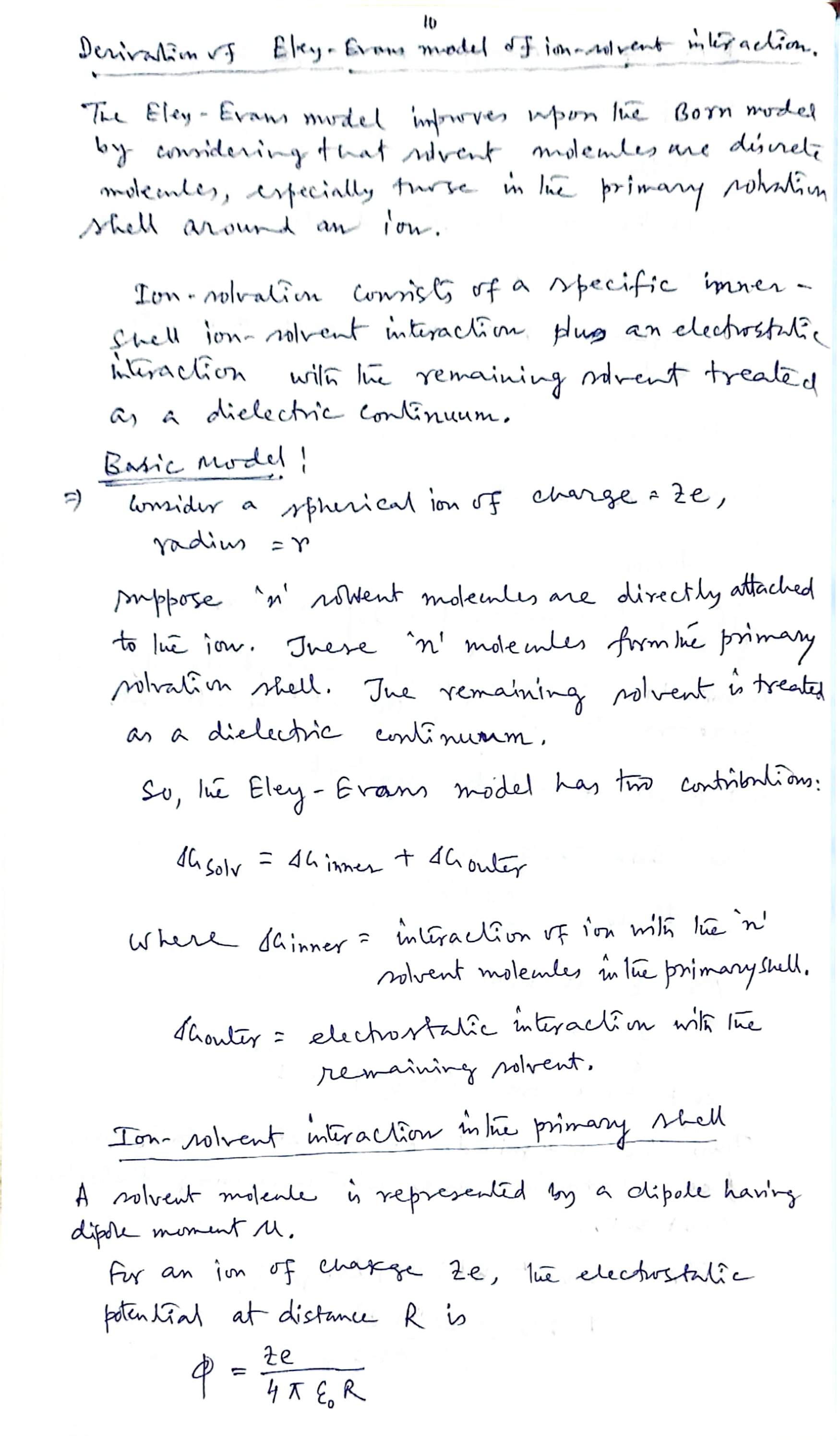
The Eley–Evans model improves upon the Born model by considering that solvent molecules are discrete molecules — especially those in the primary solvation shell around an ion. Ion solvation then consists of a specific inner-shell ion–solvent interaction plus an electrostatic interaction with the remaining solvent treated as a dielectric continuum.

Basic model

Consider a spherical ion of charge $ze$ and radius $r$ . Suppose $n$ solvent molecules are directly attached to the ion; these $n$ molecules form the primary solvation shell. The remaining solvent is treated as a dielectric continuum. So the Eley–Evans model has two contributions:

\Delta G_{\text{solv}} = \Delta G_{\text{inner}} + \Delta G_{\text{outer}}

$\Delta G_{\text{inner}}$ = interaction of the ion with the $n$ solvent molecules in the primary shell,
$\Delta G_{\text{outer}}$ = electrostatic interaction with the remaining solvent.

Schematic representation: central ion of charge ze surrounded by a primary solvation shell of n solvent molecules at distance R; the outer region is treated as a dielectric continuum with dielectric constant epsilon — **The Eley–Evans picture** (printed schematic from the lecture). Central ion (charge $ze$ ); ● = O atom of solvent molecule, ○ = H atom of solvent molecule; $R$ = distance between ion and solvent molecule. Inner dashed circle: **primary solvation shell** ( $n$ molecules). Outer dashed circle: region treated as a **dielectric continuum** (dielectric constant $=\varepsilon$ ).

05 Inner-shell contribution: ion–dipole interaction

A solvent molecule in the primary shell is represented by a dipole having dipole moment $\mu$ . For an ion of charge $ze$ , the electrostatic potential at distance $R$ is

\phi = \frac{ze}{4\pi\varepsilon_0 R}

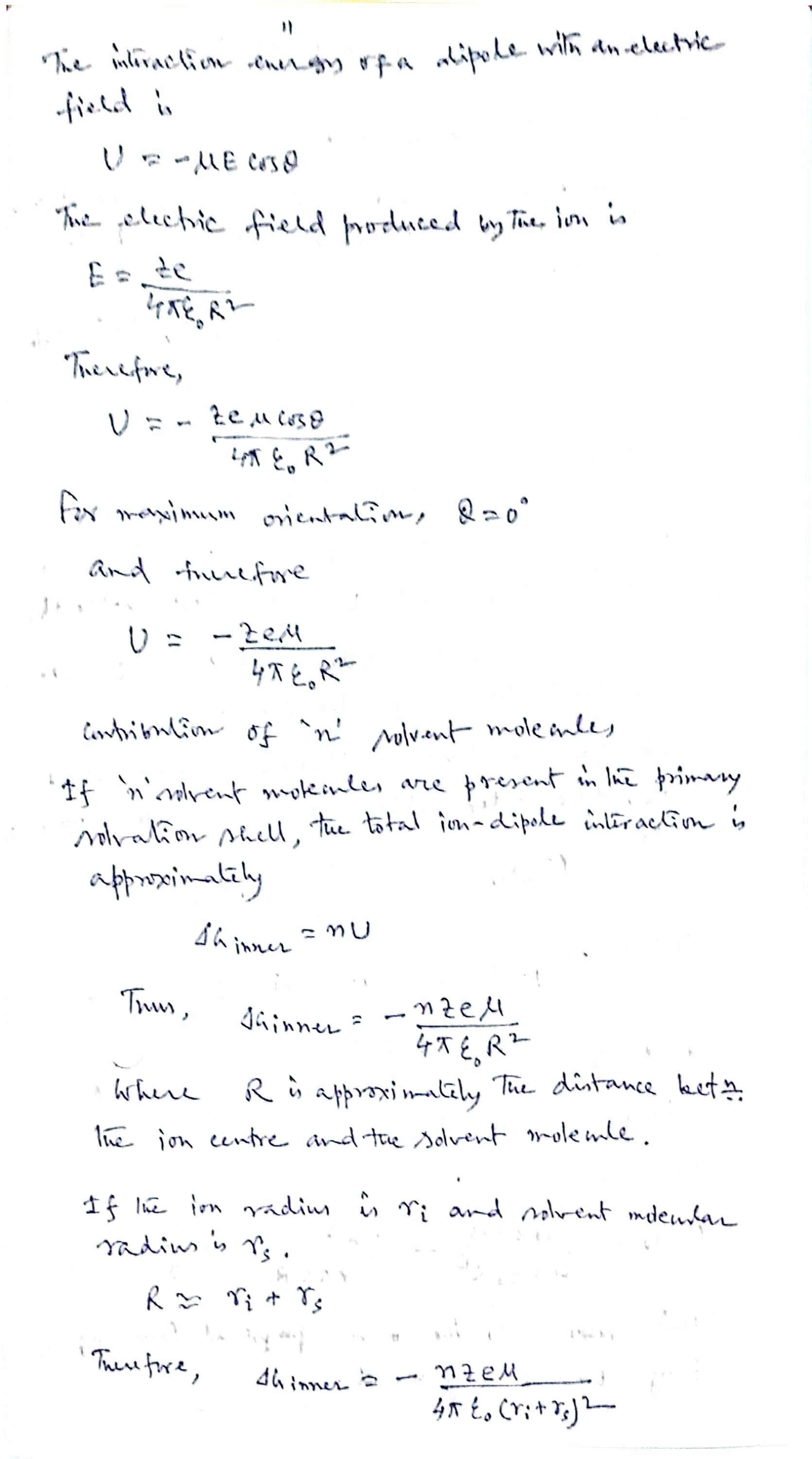
The interaction energy of a dipole with an electric field is $U = -\mu E \cos\theta$ ; the electric field produced by the ion is

E = \frac{ze}{4\pi\varepsilon_0 R^2}

Therefore,

vii

U = -\frac{ze\,\mu\cos\theta}{4\pi\varepsilon_0 R^2}

For maximum orientation, $\theta = 0^\circ$ and therefore $\cos\theta = 1$ :

viii

U = -\frac{ze\,\mu}{4\pi\varepsilon_0 R^2}

Contribution of n solvent molecules

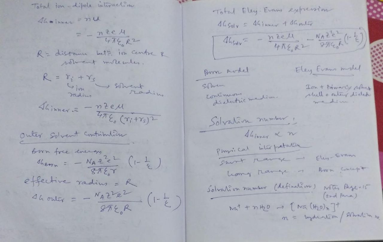
If $n$ solvent molecules are present in the primary solvation shell, the total ion–dipole interaction is approximately

\Delta G_{\text{inner}} = nU = -\frac{n\,ze\,\mu}{4\pi\varepsilon_0 R^2}

where $R$ is approximately the distance between the ion centre and the solvent molecule. If the ion radius is $r_i$ and the solvent-molecule radius is $r_s$ , then $R \simeq r_i + r_s$ , and therefore

\Delta G_{\text{inner}} = -\frac{n\,ze\,\mu}{4\pi\varepsilon_0\,(r_i + r_s)^2}

06 Outer-shell contribution & the total Eley–Evans equation

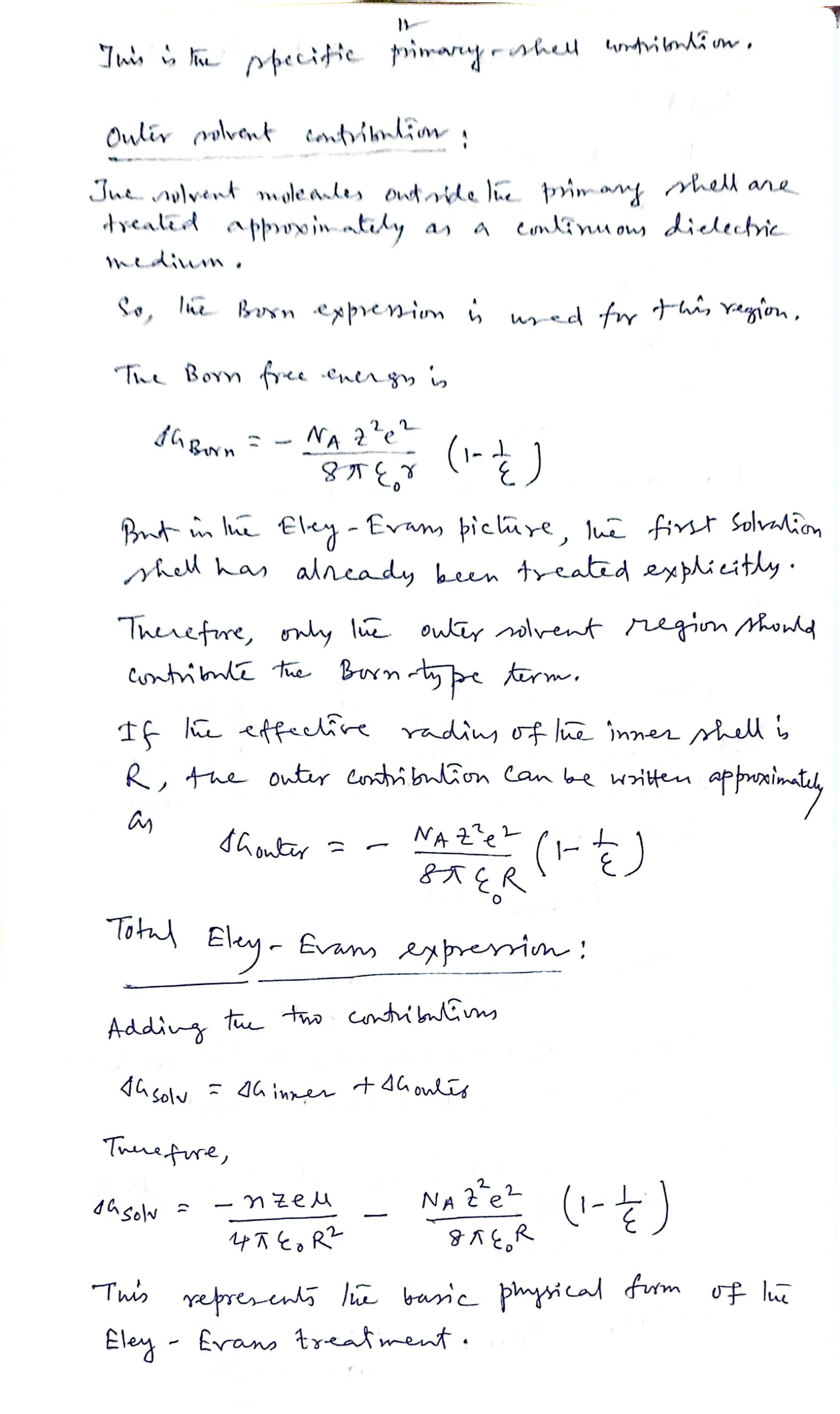
The solvent molecules outside the primary shell are treated approximately as a continuous dielectric medium, so the Born expression is used for this region. The Born free energy is (Class 1, Section 5):

\Delta G_{\text{Born}} = -\frac{N_A\, z^2 e^2}{8\pi\varepsilon_0\, r}\left(1 - \frac{1}{\varepsilon}\right)

But in the Eley–Evans picture the first solvation shell has already been treated explicitly; therefore only the outer solvent region should contribute the Born-type term. If the effective radius of the inner shell is $R$ , the outer contribution can be written approximately as

xii

\Delta G_{\text{outer}} = -\frac{N_A\, z^2 e^2}{8\pi\varepsilon_0\, R}\left(1 - \frac{1}{\varepsilon}\right)

Total Eley–Evans expression

Adding the two contributions, $\Delta G_{\text{solv}} = \Delta G_{\text{inner}} + \Delta G_{\text{outer}}$ ; therefore

xiii

\Delta G_{\text{solv}} = -\frac{n\,ze\,\mu}{4\pi\varepsilon_0 R^2} - \frac{N_A\, z^2 e^2}{8\pi\varepsilon_0\, R}\left(1 - \frac{1}{\varepsilon}\right)

This represents the basic physical form of the Eley–Evans treatment.

Unit check — the Nₐ trap again (cf. Class 1, Section 5)

Exactly as boxed in the notebook, the inner term is the energy of one ion with its $n$ dipoles, while the outer Born term is per mole (it carries $N_A$ ). Put on a single molar footing the equation reads $\Delta G_{\text{solv}} = -\frac{N_A\, n\, z e\, \mu}{4\pi\varepsilon_0 R^2} - \frac{N_A\, z^2 e^2}{8\pi\varepsilon_0\, R}\left(1 - \frac{1}{\varepsilon}\right)$ . Keep the notebook's boxed form for the exam, but state which footing you are on — adding a per-ion term to a per-mole term in one sum is the easiest way to lose marks here.

Relation with the solvation number

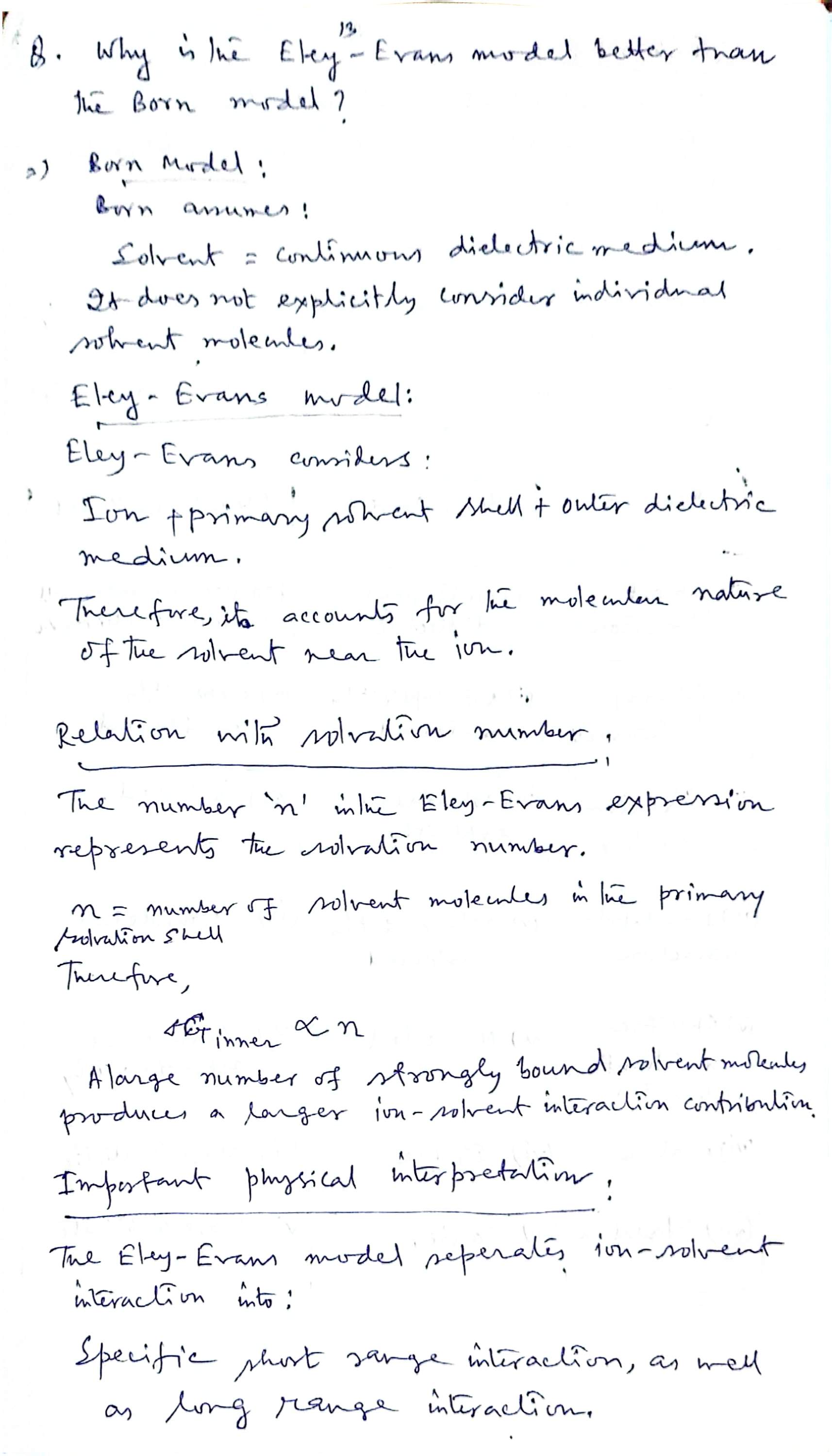
The number $n$ appearing in the Eley–Evans expression is the solvation number — the number of solvent molecules in the primary / solvation shell. Since $\Delta G_{\text{inner}} \propto n$ , a large number of strongly bound solvent molecules produces a larger ion–solvent interaction contribution.

visual lab 4

Eley–Evans cutaway: two regions, two terms

Born sees one grey continuum. Eley–Evans cuts it in two: a molecular inner shell and a continuum outside it. Switch the highlight to see which region each term of the boxed equation comes from.

ΔG(solv) = − n·z·e·μ / (4π·ε0·R²) − (N_A·z²·e² / 8π·ε0·R)·(1 − 1/ε)the notebook's boxed total — see the Section 6 unit-check for the N_A footing

The shell dipoles wobble toward θ = 0° (maximum orientation, Section 5) and the continuum starts outside the primary shell — count the first shell once only, with r → R in the Born term (Section 6).

07 Born vs Eley–Evans: what actually changes

Q. Why is the Eley–Evans model better than the Born model? Born assumes: solvent = continuous dielectric medium; it does not explicitly consider individual solvent molecules. Eley–Evans considers: ion + primary solvent shell + outer dielectric medium — therefore it accounts for the molecular nature of the solvent near the ion.

Important physical interpretation: two ranges

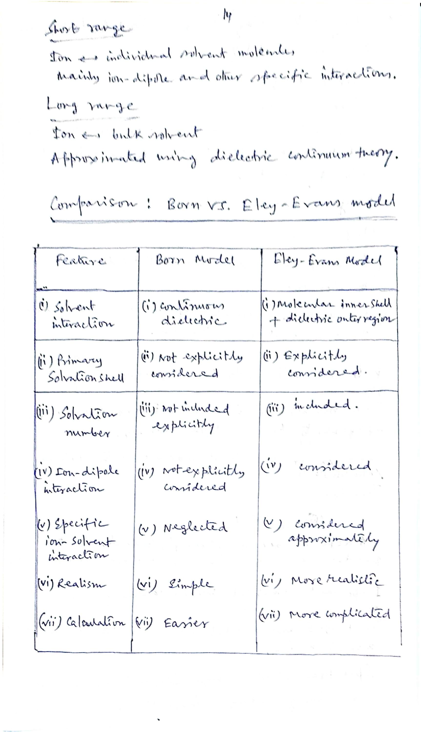
Short range: ion ↔ individual solvent molecules — mainly ion–dipole and other specific interactions (the Eley–Evans inner term).
Long range: ion ↔ bulk solvent — approximated using dielectric continuum theory (the Born concept).

Feature	Born model	Eley–Evans model
(i) Solvent interaction	continuous dielectric	molecular inner shell + dielectric outer region
(ii) Primary solvation shell	not explicitly considered	explicitly considered
(iii) Solvation number	not included explicitly	included
(iv) Ion–dipole interaction	not explicitly considered	considered
(v) Specific ion–solvent interaction	neglected	considered approximately
(vi) Realism	simple	more realistic
(vii) Calculation	easier	more complicated

08 Method 1 · Density / apparent molar volume

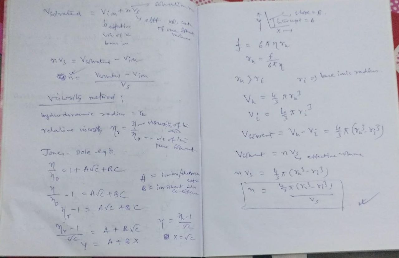
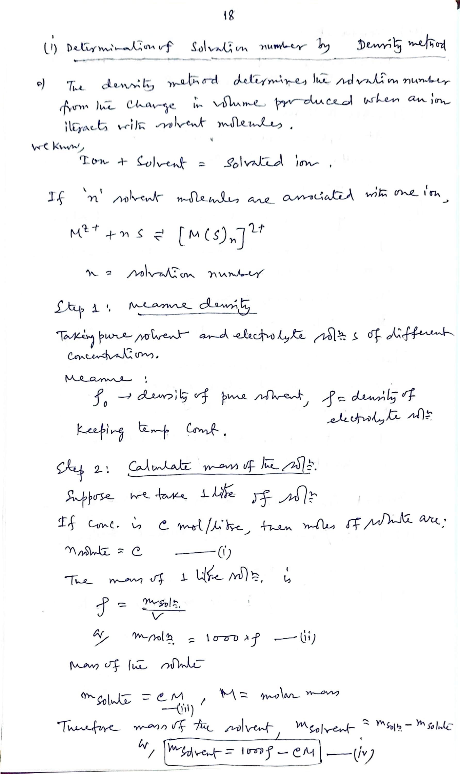
The density method determines the solvation number from the change in volume produced when an ion interacts with solvent molecules. We know: ion + solvent = solvated ion; if $n$ solvent molecules are associated with one ion, $\mathrm{M}^{z+} + n\,\mathrm{S} \rightleftharpoons [\mathrm{M(S)}_n]^{z+}$ (eq. ii), with $n$ = solvation number.

Measure density

Take pure solvent and electrolyte solutions of different concentrations. Measure: $\rho_0$ = density of pure solvent, $\rho$ = density of electrolyte solution — keeping temperature constant.

Calculate mass of the solution (take 1 litre)

If the concentration is $c$ mol L⁻¹ then the moles of solute are $n_{\text{solute}} = c$ …(i). The mass of 1 litre of solution: $\rho = m_{\text{soln}}/V \Rightarrow m_{\text{soln}} = 1000 \times \rho$ …(ii). Mass of the solute: $m_{\text{solute}} = cM$ …(iii), where $M$ = molar mass. Therefore the mass of the solvent, $m_{\text{solvent}} = m_{\text{soln}} - m_{\text{solute}}$ :

xiv

m_{\text{solvent}} = 1000\,\rho - cM

Calculate volume of solvent

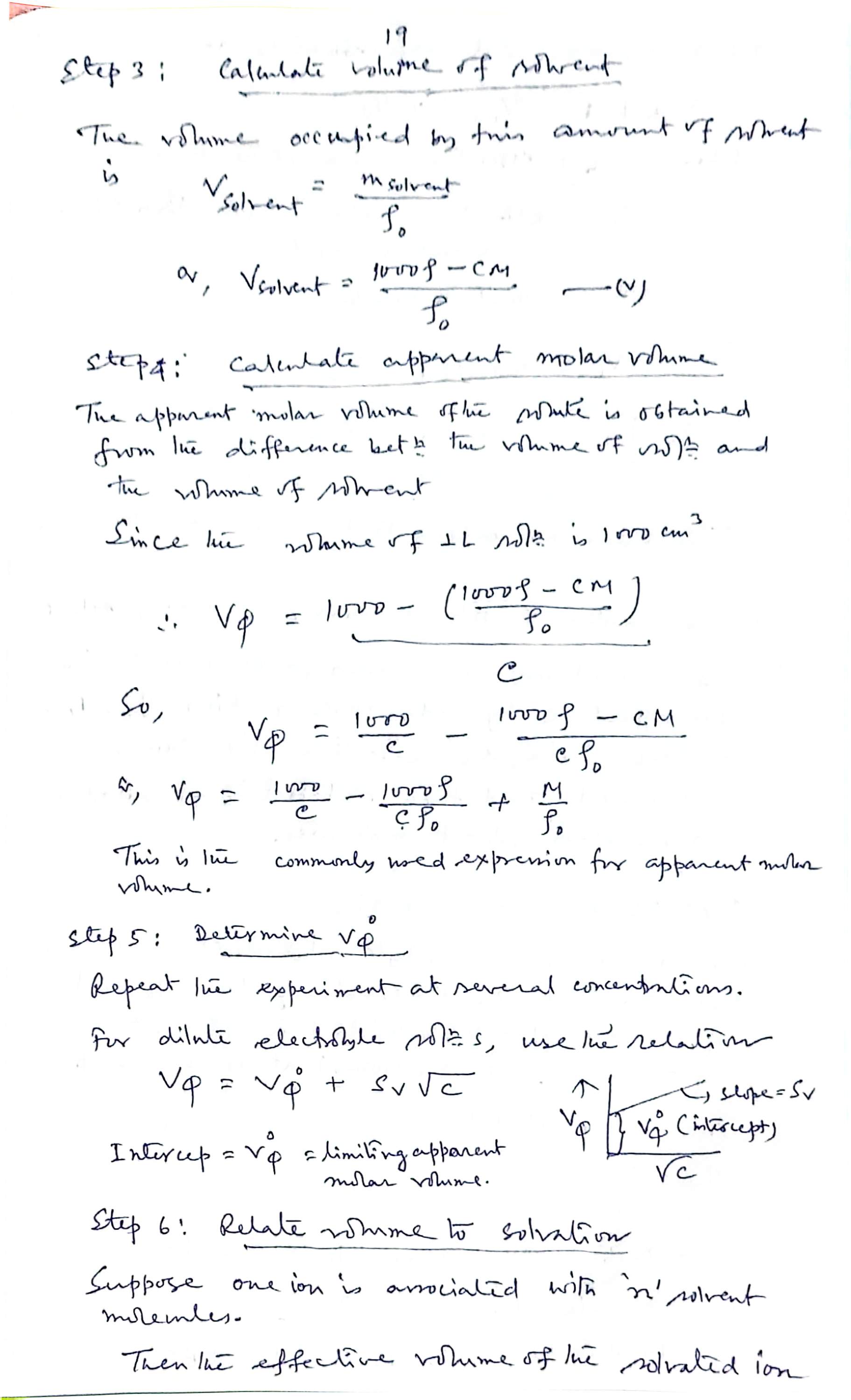
The volume occupied by this amount of solvent is $V_{\text{solvent}} = m_{\text{solvent}}/\rho_0$ :

V_{\text{solvent}} = \frac{1000\,\rho - cM}{\rho_0}

Calculate apparent molar volume

The apparent molar volume of the solute is obtained from the difference between the volume of solution and the volume of solvent. Since the volume of 1 L of solution is 1000 cm³:

xvi

V_\phi = \frac{1000 - \left(\dfrac{1000\,\rho - cM}{\rho_0}\right)}{c} = \frac{1000}{c} - \frac{1000\,\rho - cM}{c\,\rho_0}

xvii

V_\phi = \frac{1000}{c} - \frac{1000\,\rho}{c\,\rho_0} + \frac{M}{\rho_0}

This is the commonly used expression for the apparent molar volume.

Determine V_φ° (limiting apparent molar volume)

Repeat the experiment at several concentrations. For dilute electrolyte solutions, use the relation

xviii

V_\phi = V_\phi^{\circ} + S_V \sqrt{c}

Plot $V_\phi$ against $\sqrt{c}$ : the intercept $= V_\phi^{\circ}$ = limiting apparent molar volume, the slope $= S_V$ .

Relate volume to solvation

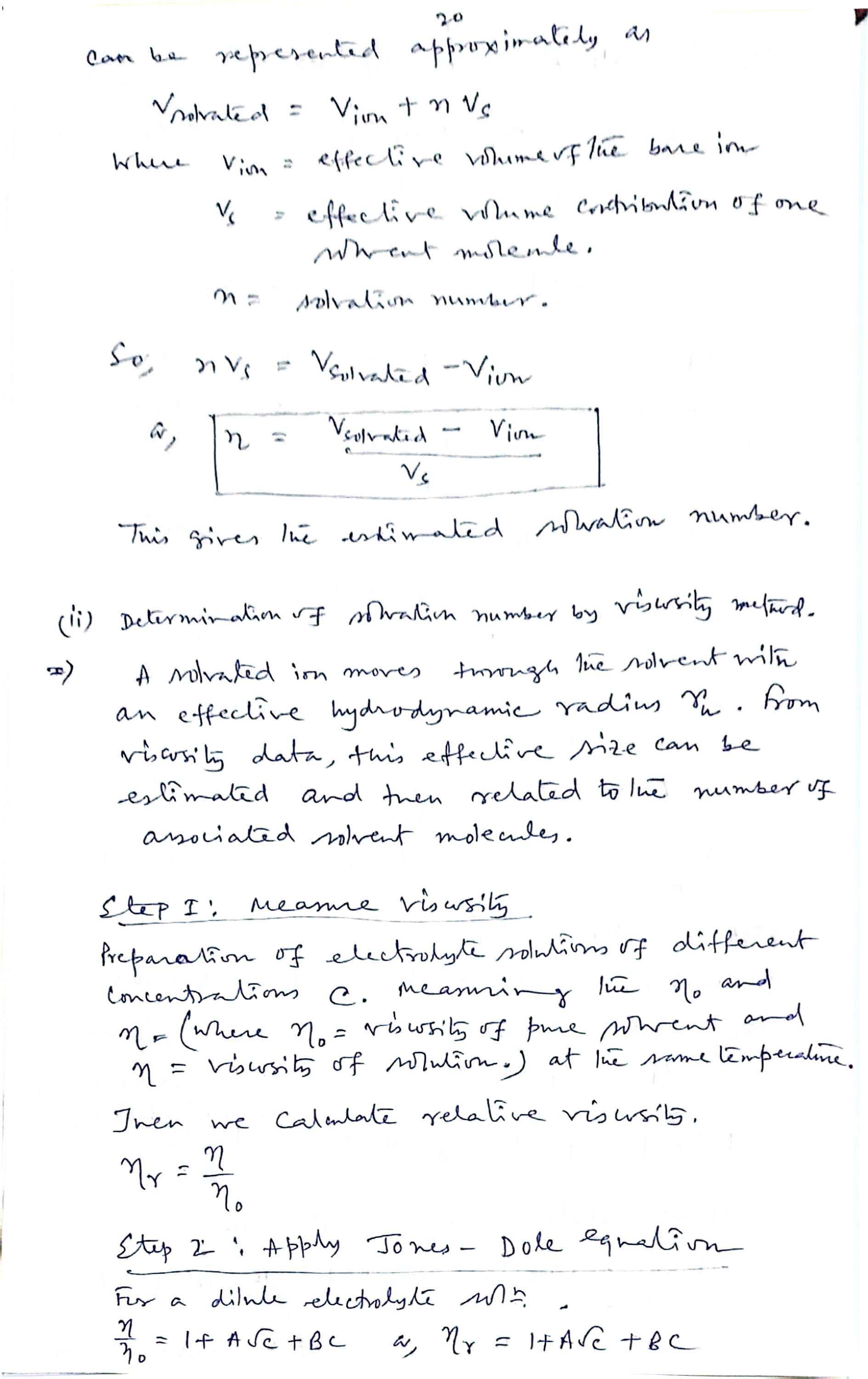
Suppose one ion is associated with $n$ solvent molecules. Then the effective volume of the solvated ion can be represented approximately as

xix

V_{\text{solvated}} = V_{\text{ion}} + n\,V_s

where $V_{\text{ion}}$ = effective volume of the bare ion and $V_s$ = effective volume contribution of one solvent molecule. So $n V_s = V_{\text{solvated}} - V_{\text{ion}}$ :

n = \frac{V_{\text{solvated}} - V_{\text{ion}}}{V_s}

This gives the estimated solvation number.

09 Method 2 · Viscosity (Jones–Dole → hydrodynamic radius)

A solvated ion moves through the solvent with an effective hydrodynamic radius $r_h$ . From viscosity data this effective size can be estimated and then related to the number of associated solvent molecules.

Measure viscosity

Prepare electrolyte solutions of different concentrations $c$ ; measure $\eta_0$ and $\eta$ , where $\eta_0$ = viscosity of pure solvent and $\eta$ = viscosity of solution, at the same temperature. Then the relative viscosity is $\eta_r = \eta/\eta_0$ .

Apply the Jones–Dole equation

For a dilute electrolyte solution:

xxi

\frac{\eta}{\eta_0} = \eta_r = 1 + A\sqrt{c} + Bc

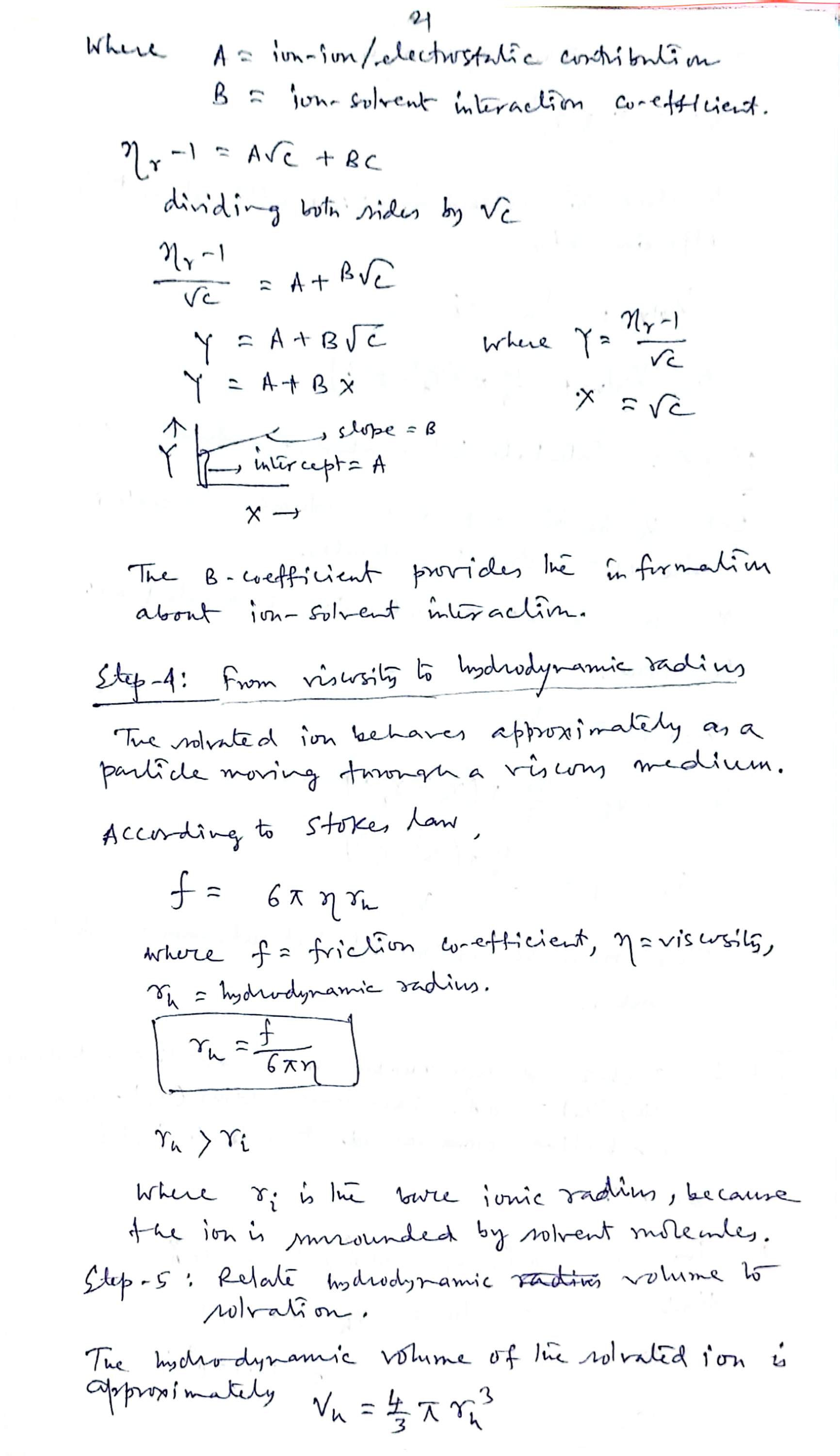
where $A$ = ion–ion / electrostatic contribution and $B$ = ion–solvent interaction coefficient.

Linearise and plot

$\eta_r - 1 = A\sqrt{c} + Bc$ ; dividing both sides by $\sqrt{c}$ :

xxii

\frac{\eta_r - 1}{\sqrt{c}} = A + B\sqrt{c} \quad\Longrightarrow\quad Y = A + BX,\ \ Y = \frac{\eta_r - 1}{\sqrt{c}},\ \ X = \sqrt{c}

Plot $Y$ vs $X$ : intercept $= A$ , slope $= B$ . The $B$ -coefficient provides the information about ion–solvent interaction.

From viscosity to hydrodynamic radius (Stokes)

The solvated ion behaves approximately as a particle moving through a viscous medium. According to Stokes' law, $f = 6\pi\eta r_h$ , where $f$ = friction coefficient, $\eta$ = viscosity, $r_h$ = hydrodynamic radius:

xxiii

r_h = \frac{f}{6\pi\eta}

and $r_h > r_i$ , where $r_i$ is the bare ionic radius, because the ion is surrounded by solvent molecules.

Hydrodynamic volumes

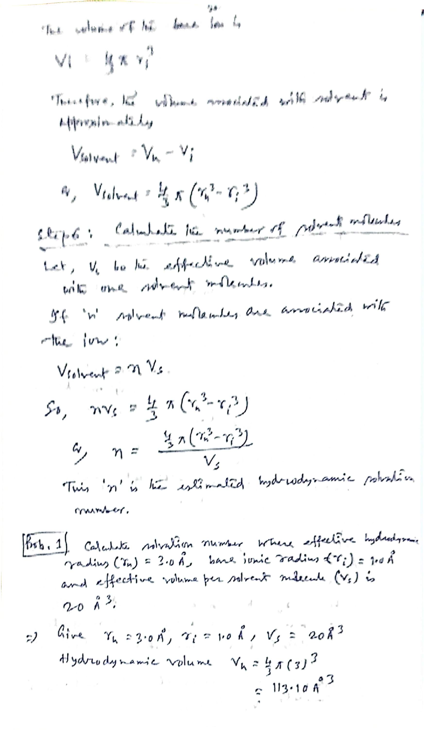
The hydrodynamic volume of the solvated ion is approximately $V_h = \tfrac{4}{3}\pi r_h^3$ ; the volume of the bare ion is $V_i = \tfrac{4}{3}\pi r_i^3$ . Therefore the volume associated with solvent is

xxiv

V_{\text{solvent}} = V_h - V_i = \frac{4}{3}\pi\left(r_h^3 - r_i^3\right)

Calculate the number of solvent molecules

Let $V_s$ be the effective volume associated with one solvent molecule. If $n$ solvent molecules are associated with the ion, $V_{\text{solvent}} = n V_s$ , so $n V_s = \tfrac{4}{3}\pi(r_h^3 - r_i^3)$ :

xxv

n = \frac{\tfrac{4}{3}\pi\left(r_h^3 - r_i^3\right)}{V_s}

This $n$ is the estimated hydrodynamic solvation number.

visual lab 5

The straight line that both methods rely on

Dilute-solution data are useless until you linearise them. Drag the intercept and slope and watch what the experiment actually extracts: intercept = ion-free limit, slope = the interaction you care about.

intercept A — 0.25

slope B — 0.60

(ηr − 1)/√c = 0.25 + 0.60·√c

Jones–Dole: the intercept A is the ion–ion / electrostatic piece, the slope B is the ion–solvent interaction coefficient (Section 9). Apparent molar volume: intercept V_φ° is the limiting apparent molar volume, slope S_V (Section 8, step 5). Same mathematics, two experiments.

10 Method 3 · Conductance / ionic mobility

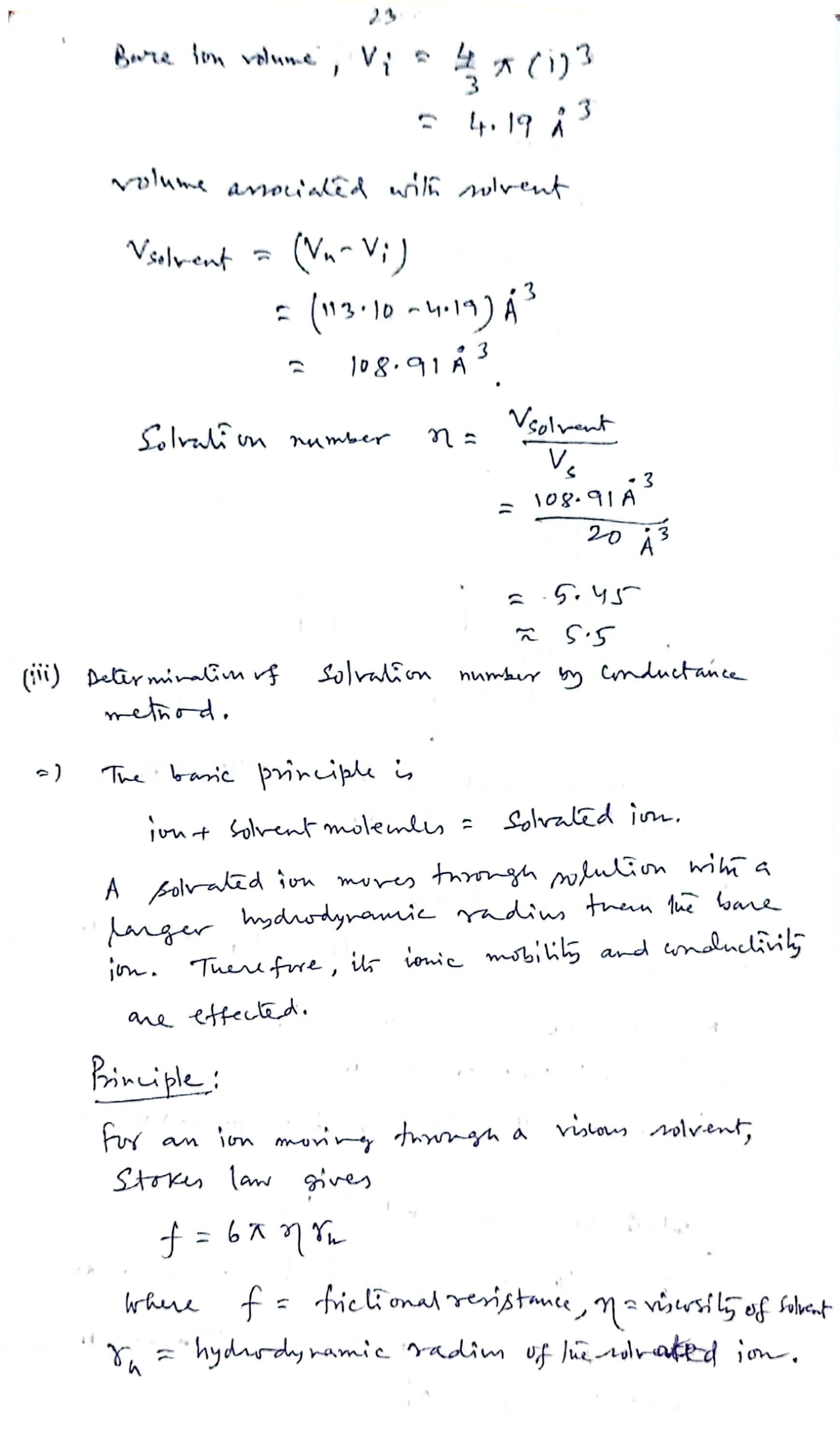
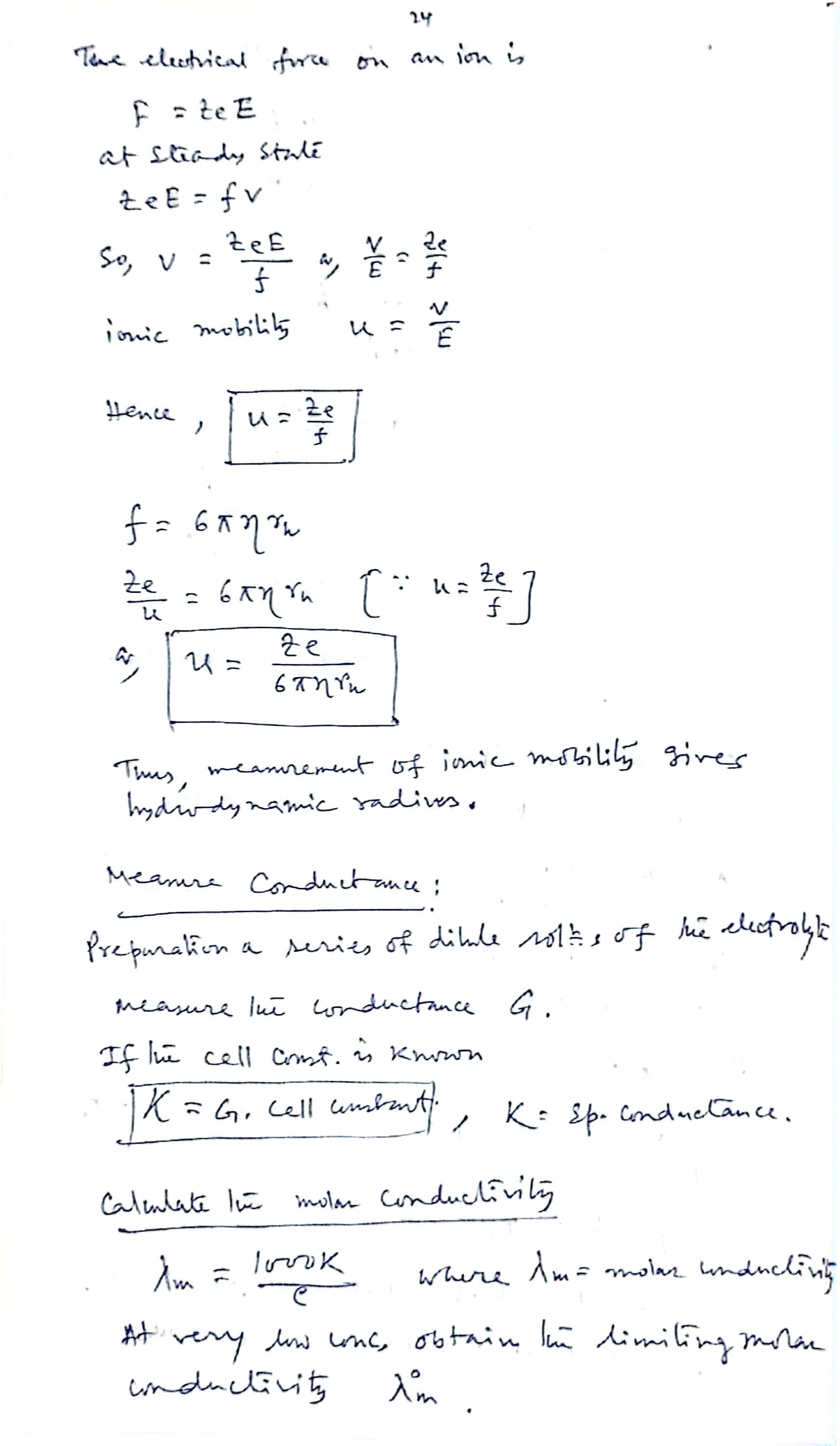
Basic principle: ion + solvent molecules = solvated ion. A solvated ion moves through solution with a larger hydrodynamic radius than the bare ion; therefore its ionic mobility and conductivity are affected. For an ion moving through a viscous solvent, Stokes' law gives $f = 6\pi\eta r_h$ , where $f$ = frictional resistance, $\eta$ = viscosity of solvent, $r_h$ = hydrodynamic radius of the solvated ion.

From mobility to radius

The electrical force on an ion is $F = zeE$ ; at steady state $zeE = fv$ , so $v = zeE/f$ and $v/E = ze/f$ . The ionic mobility is $u = v/E$ ; hence $u = ze/f$ , and with $f = 6\pi\eta r_h$ :

xxvi

u = \frac{ze}{6\pi\eta\, r_h}

Thus, measurement of ionic mobility gives the hydrodynamic radius.

Measure conductance

Prepare a series of dilute solutions of the electrolyte; measure the conductance $G$ .
If the cell constant is known: $\kappa = G \times (\text{cell constant})$ , where $\kappa$ = specific conductance.
Molar conductivity: $\lambda_m = \dfrac{1000\,\kappa}{c}$ ; at very low concentration obtain the limiting molar conductivity $\lambda_m^{\circ}$ .
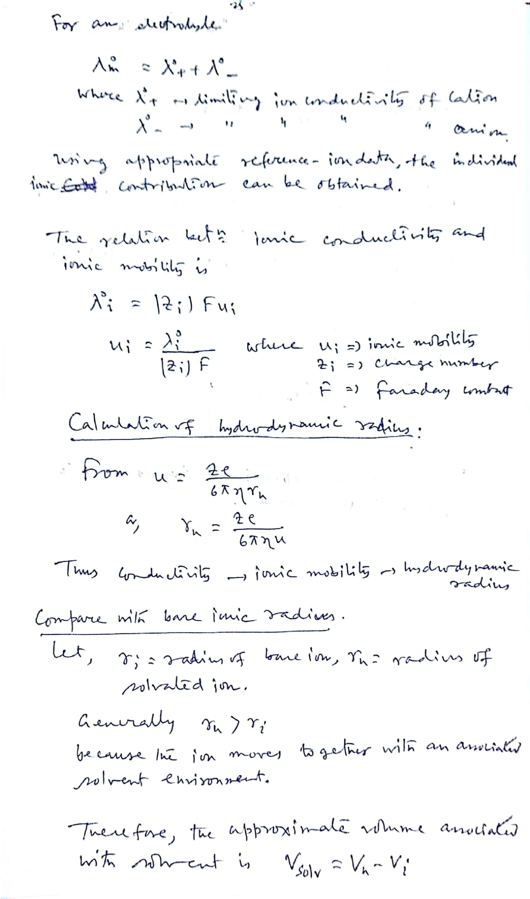
For an electrolyte: $\lambda_m^{\circ} = \lambda_+^{\circ} + \lambda_-^{\circ}$ ; using appropriate reference-ion data, the individual ionic contributions can be obtained.

Ionic conductivity ↔ ionic mobility

xxvii

\lambda_i^{\circ} = \lvert z_i \rvert\, F\, u_i \quad\Longrightarrow\quad u_i = \frac{\lambda_i^{\circ}}{\lvert z_i \rvert\, F}

where $u_i$ = ionic mobility, $z_i$ = charge number, $F$ = Faraday constant.

Hydrodynamic radius, then n

From $u = ze/(6\pi\eta r_h)$ :

xxviii

r_h = \frac{ze}{6\pi\eta\, u}

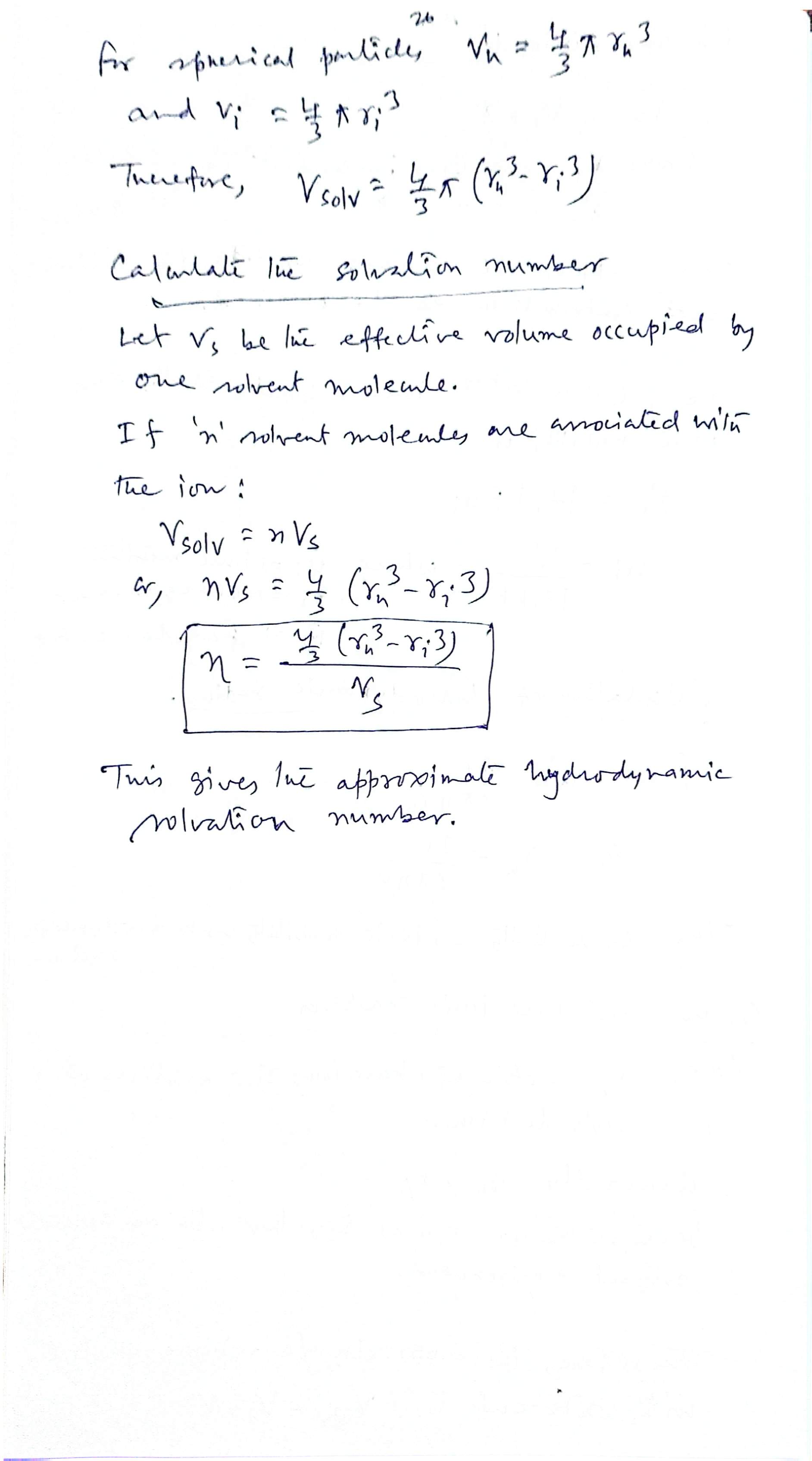
Thus: conductivity → ionic mobility → hydrodynamic radius. Compare with the bare ionic radius: let $r_i$ = radius of bare ion, $r_h$ = radius of solvated ion. Generally $r_h > r_i$ , because the ion moves together with an associated solvent environment. Therefore the approximate volume associated with solvent is $V_{\text{solv}} = V_h - V_i$ ; for spherical particles $V_h = \tfrac{4}{3}\pi r_h^3$ and $V_i = \tfrac{4}{3}\pi r_i^3$ , so $V_{\text{solv}} = \tfrac{4}{3}\pi(r_h^3 - r_i^3)$ . Let $V_s$ be the effective volume occupied by one solvent molecule; if $n$ solvent molecules are associated with the ion, $V_{\text{solv}} = n V_s$ :

xxix

n = \frac{\tfrac{4}{3}\pi\left(r_h^3 - r_i^3\right)}{V_s}

This gives the approximate hydrodynamic solvation number from transport data.

visual lab 6

Mobility race: who drags the shell pays for it

Two identical charges in the same field E, same solvent viscosity η. Top lane: the bare ion (radius r_i). Bottom lane: the same ion wearing its hydrodynamic shell (radius r_h > r_i). Stokes says the shelled one drifts slower by exactly r_i/r_h.

bare radius r(i) (Å) — 1.0

shell thickness (Å) — 2.0

r(h) = 3.0 Å u(solv)/u(bare) = r(i)/r(h) = 0.33 u = ze/(6π·η·r(h)) → bigger shell, slower drift

This slowdown is precisely what the conductance method measures: conductivity → ionic mobility u → hydrodynamic radius r(h) = ze/(6π·η·u) → solvation number n (Section 10). Reduced-motion users: set the sliders and read the ratio — the physics is in the numbers, not the animation.

11 Play with the solvation number

The boxed hydrodynamic formula, live: punch in the hydrodynamic radius, the bare ionic radius and the effective volume per solvent molecule — the calculator returns the shell volumes and the solvation number n (viscosity & conductance routes, Sections 9–10).

Hydrodynamic radius r_h (Å)

Bare ionic radius r_i (Å)

Volume per solvent molecule V_s (Å³)

V(h) = 4/3 π r(h)³

113.10 Å³

V(i) = 4/3 π r(i)³

4.19 Å³

V(solvent) = V(h) − V(i)

108.91 Å³

solvation number n

5.45 ≈ 5.5

Try r_h = 3.0 Å, r_i = 1.0 Å, V_s = 20 Å³: you should recover the lecture's Prob. 1 — V(h) = 113.10 Å³, V(i) = 4.19 Å³, V(solvent) = 108.91 Å³, n = 5.45 ≈ 5.5. Remember n is a hydrodynamic estimate: it counts every solvent molecule that moves with the ion, so it sits at the high end of the primary-shell counts (Section 1).

12 The equation sheet, at a glance

Every boxed result of the lecture on one screen. Labels match the derivation above.

viii

U = -\frac{ze\,\mu}{4\pi\varepsilon_0 R^2}

\Delta G_{\text{inner}} = -\frac{n\,ze\,\mu}{4\pi\varepsilon_0\,(r_i + r_s)^2}

xii

\Delta G_{\text{outer}} = -\frac{N_A\, z^2 e^2}{8\pi\varepsilon_0\, R}\left(1 - \frac{1}{\varepsilon}\right)

xiii

\Delta G_{\text{solv}} = -\frac{n\,ze\,\mu}{4\pi\varepsilon_0 R^2} - \frac{N_A\, z^2 e^2}{8\pi\varepsilon_0\, R}\left(1 - \frac{1}{\varepsilon}\right)

xiv

m_{\text{solvent}} = 1000\,\rho - cM

xvii

V_\phi = \frac{1000}{c} - \frac{1000\,\rho}{c\,\rho_0} + \frac{M}{\rho_0}

xviii

V_\phi = V_\phi^{\circ} + S_V \sqrt{c}

n = \frac{V_{\text{solvated}} - V_{\text{ion}}}{V_s}

xxi

\eta_r = \frac{\eta}{\eta_0} = 1 + A\sqrt{c} + Bc

xxiii

r_h = \frac{f}{6\pi\eta}

xxv

n = \frac{\tfrac{4}{3}\pi\left(r_h^3 - r_i^3\right)}{V_s}

xxvi

u = \frac{ze}{6\pi\eta\, r_h}

xxvii

\lambda_i^{\circ} = \lvert z_i \rvert\, F\, u_i

13 Symbol table

Symbol	Meaning	Typical unit
$n$	Solvation (hydration) number — solvent molecules in the primary shell	dimensionless
$z$ , $z_i$	Charge number of the ion	dimensionless
$e$	Elementary charge	C
$\mu$	Dipole moment of a solvent molecule	C m (1 D = 3.336 × 10⁻³⁰ C m)
$\varepsilon_0$ , $\varepsilon$	Vacuum permittivity; relative permittivity (dielectric constant) of the solvent	F m⁻¹; dimensionless
$r$ , $r_i$	Radius of the (bare) ion	m, Å
$r_s$	Radius of a solvent molecule	Å
$R$	Ion-centre → solvent-molecule distance; effective radius of the inner shell ( $R \simeq r_i + r_s$ )	m, Å
$r_h$	Hydrodynamic radius of the solvated ion ( $r_h > r_i$ )	m, Å
$\phi$ , $E$	Electrostatic potential and field of the ion at distance $R$	V; V m⁻¹
$U$	Ion–dipole interaction energy (one dipole, maximally oriented)	J
$\theta$	Angle between dipole and field (max orientation: $\theta = 0^\circ$ )	deg
$N_A$	Avogadro constant	mol⁻¹
$\Delta G_{\text{inner}}, \Delta G_{\text{outer}}$	Primary-shell (ion–dipole) and outer-continuum (Born-type) contributions	J (ion⁻¹) ; J mol⁻¹
$\rho_0$ , $\rho$	Density of pure solvent; density of electrolyte solution	g cm⁻³
$c$	Molar concentration of the electrolyte	mol L⁻¹
$M$	Molar mass of the solute	g mol⁻¹
$m_{\text{soln}}, m_{\text{solute}}, m_{\text{solvent}}$	Masses of solution (1 L), solute, solvent	g
$V_\phi$ , $V_\phi^{\circ}$ , $S_V$	Apparent molar volume; its limiting value; experimental slope vs $\sqrt{c}$	cm³ mol⁻¹
$V_{\text{solvated}}, V_{\text{ion}}, V_s$	Effective volumes: solvated ion; bare ion; one solvent molecule	cm³, Å³
$V_h$ , $V_i$ , $V_{\text{solvent}}$	Hydrodynamic volume; bare-ion volume; volume associated with solvent ( $V_h - V_i$ )	Å³
$\eta$ , $\eta_0$ , $\eta_r$	Viscosity of solution; of pure solvent; relative viscosity $\eta/\eta_0$	P / mPa s; —
$A$ , $B$	Jones–Dole coefficients: ion–ion (electrostatic); ion–solvent interaction	L¹ᐟ² mol⁻¹ᐟ²; L mol⁻¹
$f$	Friction coefficient / frictional resistance (Stokes)	kg s⁻¹
$u$ , $u_i$	Ionic mobility	m² V⁻¹ s⁻¹
$G$ , $\kappa$	Conductance; specific conductance ( $\kappa = G \times$ cell constant)	S; S m⁻¹
$\lambda_m$ , $\lambda_m^{\circ}$ , $\lambda_i^{\circ}$	Molar conductivity; limiting molar conductivity; limiting ionic conductivity	S cm² mol⁻¹
$F$	Faraday constant	C mol⁻¹

14 Rapid revision — 14 lines before the exam

Solvation number $n$ = solvent molecules in the primary shell; in water = hydration number; $\mathrm{Na}^+ + n\,\mathrm{H_2O} \to [\mathrm{Na(H_2O)}_n]^+$ .
Primary shell = strongly, directly coordinated; secondary shell = less strongly oriented → the measured $n$ depends on the definition and on the method's shell sensitivity.
$n$ grows with charge density (small $r$ , high $z$ ); solvent ε, μ, donor/acceptor ability, size and H-bonding matter; $T \uparrow$ → looser shell; high $c$ → shells overlap.
Solvent exchange $\text{Ion–Solv}_1 + \text{Solv}_2 \rightleftharpoons \text{Ion–Solv}_2 + \text{Solv}_1$ → $n$ is an average coordination number, and methods disagree slightly.
Eley–Evans = discrete inner shell (ion–dipole) + Born continuum outside: $\Delta G_{\text{solv}} = \Delta G_{\text{inner}} + \Delta G_{\text{outer}}$ .
Dipole in the ion's field: $U = -\mu E\cos\theta$ ; max at $\theta = 0^\circ$ → $U = -ze\mu/(4\pi\varepsilon_0 R^2)$ ; $\Delta G_{\text{inner}} = nU$ with $R = r_i + r_s$ .
$\Delta G_{\text{outer}}$ = Born term with $r \to R$ — the first shell must be counted once only.
Boxed total (xiii): inner per-ion term + molar Born term; on a molar footing attach $N_A$ to the inner term too.
Born vs Eley–Evans: continuum vs molecular inner shell; $n$ absent vs included; simpler vs more realistic; short range = Eley–Evans, long range = Born.
Density route: $m_{\text{solvent}} = 1000\rho - cM$ → $V_\phi = \frac{1000}{c} - \frac{1000\rho}{c\rho_0} + \frac{M}{\rho_0}$ → $V_\phi = V_\phi^\circ + S_V\sqrt{c}$ → $n = (V_{\text{solvated}} - V_{\text{ion}})/V_s$ .
Viscosity route: Jones–Dole $\eta_r = 1 + A\sqrt{c} + Bc$ ; $B$ = ion–solvent coefficient; plot $(\eta_r - 1)/\sqrt{c}$ vs $\sqrt{c}$ → intercept $A$ , slope $B$ .
Stokes bridge: $f = 6\pi\eta r_h$ → $r_h = f/(6\pi\eta)$ ; $r_h > r_i$ ; $n = \tfrac{4}{3}\pi(r_h^3 - r_i^3)/V_s$ .
Conductance route: $u = ze/(6\pi\eta r_h)$ ; $\lambda_i^\circ = \lvert z_i \rvert F u_i$ ; $r_h = ze/(6\pi\eta u)$ → same boxed $n$ .
Prob. 1 numbers: $r_h = 3.0$ Å, $r_i = 1.0$ Å, $V_s = 20$ Å³ → $V_h = 113.10$ , $V_i = 4.19$ , $V_{\text{solvent}} = 108.91$ Å³ → $n = 5.45 \approx 5.5$ .

Next up: Class 3 notes land here after the next lecture — the hub grows one page per class.

← All classes

15 Original notebook scans

Digitised from the class notebook of 22 Aug 2026 — notebook pages 10–26 (CamScanner spreads S1–S17, the fair copy) plus the in-class phone photos N1–N6; every equation above was cross-checked against these pages. Tap any thumbnail to open the full scan. (One further uploaded photo — the ΔH/ΔS derivation — is page 9 of the same notebook, i.e. Class 1 territory, so it lives on the Class 1 page as its N4 rather than being duplicated here.)

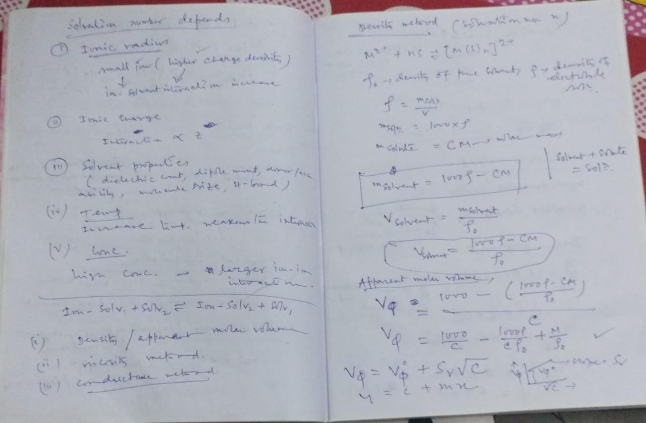N1 · factors affecting n + density method (raw)

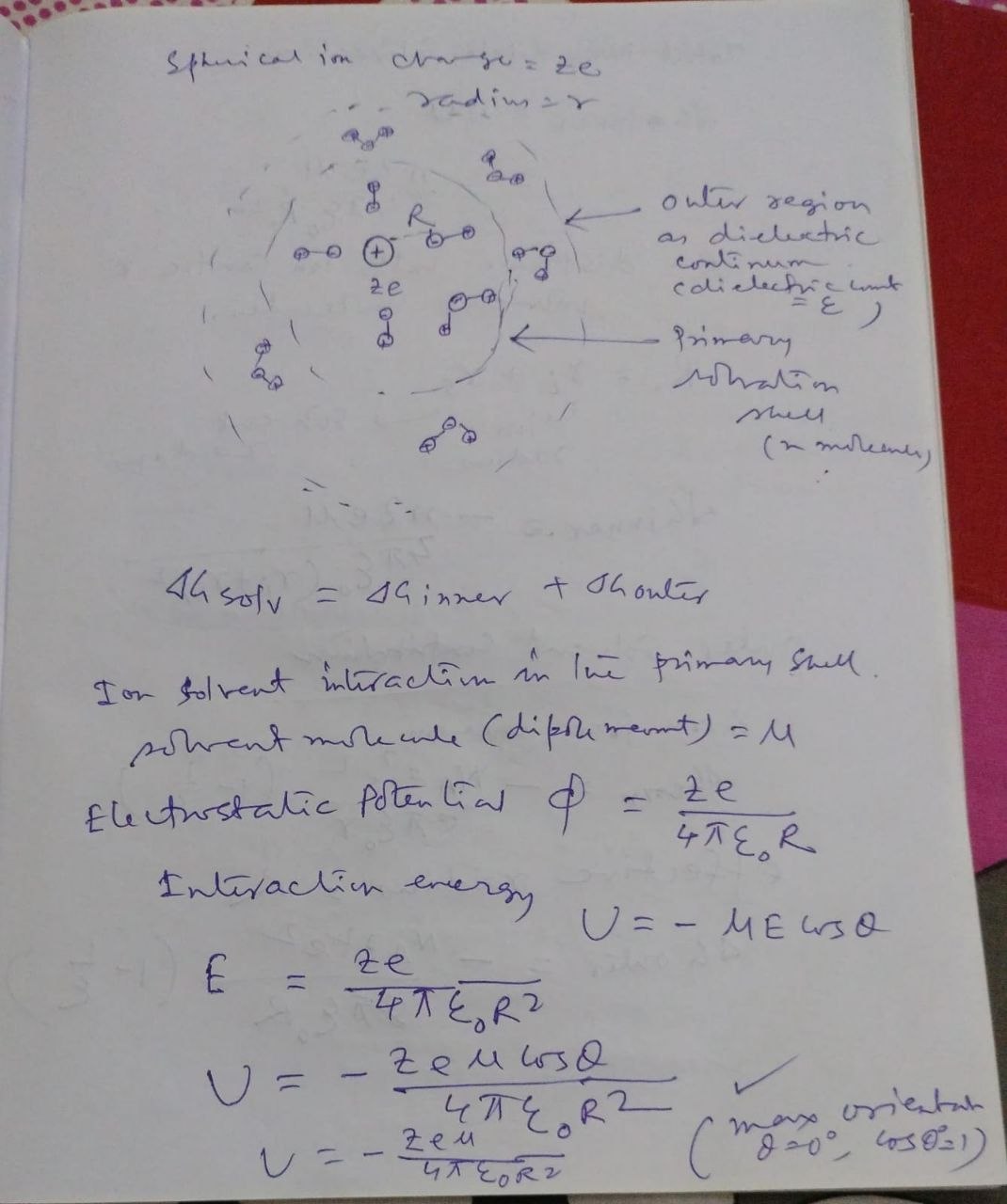N2 · primary-shell sketch, φ, E, U = −μE cosθ

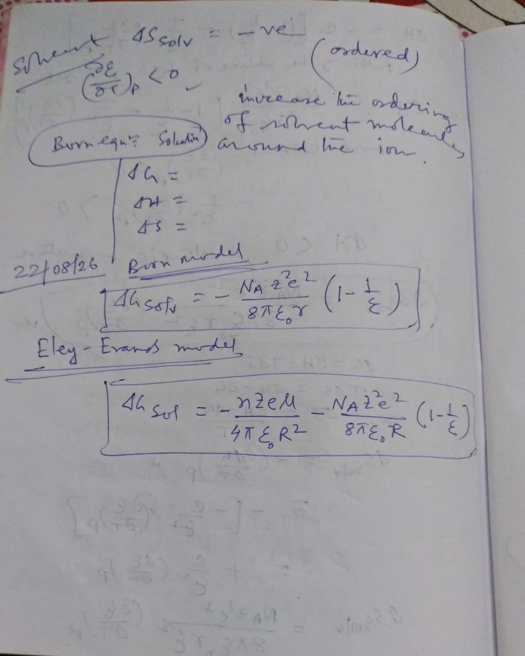N3 · 22/08/26 header, Born recap, boxed Eley–Evans

N4 · printed schematic: shell + continuum

N5 · density n, viscosity / Jones–Dole (raw)

N6 · total Eley–Evans, Born vs E-E, n defined

S1 · p10 · Eley–Evans intro, basic model, φ

S2 · p11 · U, θ = 0°, ΔG(inner) = nU

S3 · p12 · outer term + total expression

S4 · p13 · why better than Born, n ∝ ΔG(inner)

S5 · p14 · short/long range + comparison table

S6 · p15 · solvation number, primary/secondary

S7 · p16 · secondary shell, factors (i)–(iii)

S8 · p17 · factors (iv)–(v), exchange, 3 methods

S9 · p18 · density method steps 1–2

S10 · p19 · V(solvent), V(φ), V(φ)° plot

S11 · p20 · boxed n (density) + viscosity start

S12 · p21 · Jones–Dole plot, Stokes r(h)

S13 · p22 · volumes, boxed n, Prob. 1 given

S14 · p23 · Prob. 1 solved, conductance principle

S15 · p24 · u = ze/f = ze/6πηr(h), κ, λ(m)

S16 · p25 · λ° = |z|Fu, r(h) from u, r(h) > r(i)

S17 · p26 · boxed n (conductance route)

16 PYQ bank · University papers 2020–2024

Same audit as Class 1: every page of the five M.Sc. Semester-I question papers (2020, 2021, 2022, 2023, 2024 — all subjects MSCH-101…106, 60 scanned pages) was OCR'd and verified by hand. The Physical Chemistry paper each year is MSCH-104 (Physical General-I). The rule for this bank is strict: only questions that actually appeared, tagged with year and repeat count.

Year	Physical paper (MSCH-104)	Pages verified	Class-2 questions (solvation number / Eley–Evans / viscosity–conductance)
2020	Physical General I (new + old syllabus copies)	p. 12–15	0 — group theory, QM, stat-thermo, rotational/vibrational spectroscopy, fullerenes
2021	Physical General I (+ internal)	p. 7–8	0 — group theory, QM, partition functions, nanotubes, Raman
2022	Physical General I	p. 9–10	0 — symmetry, operators, spectroscopy, stat-thermo
2023	Physical General I	p. 9–10	0 — point groups, operators, rotors, Raman, fullerenes, stat-thermo
2024	Physical General I	p. 12–13	0 — group theory, matrices, rotors, polarizability, partition functions

Honest verdict

Across 2020–2024 the university never asked a solvation-number / Eley–Evans / Jones–Dole type question in these papers — in fact MSCH-104 in these years is entirely group theory, quantum mechanics, spectroscopy and statistical thermodynamics — so, per the rule, the year-tagged bank stays empty rather than being padded with look-alikes. The moment one appears in a future paper it lands here with its year and repeat count. For practice, the lecture's own exam-style questions below are answered in full, exactly as taught.

Lecture's own exam-style questions — answered in full

Lecture Q1conceptual · definitionSection 1

Q. What is the solvation number?

Ans. When an ion is introduced into a solvent, solvent molecules arrange themselves around the ion because of ion–solvent interactions. The number of solvent molecules directly associated with the ion in its primary solvation shell is the solvation number — for water, the hydration number. Example: $\mathrm{Na}^+ + n\,\mathrm{H_2O} \to [\mathrm{Na(H_2O)}_n]^+$ , where $n$ is the hydration / solvation number. Because a weaker secondary shell also exists, the measured value depends on the definition and on which shell the method senses.

Lecture Q2reasoning · experimentSection 3

Q. Why do we need experimental methods to determine the solvation number?

Ans. Ion-bound solvent molecules are not permanently fixed — they continuously exchange: $\text{Ion–Solv}_1 + \text{Solv}_2 \rightleftharpoons \text{Ion–Solv}_2 + \text{Solv}_1$ . Hence the solvation number is generally an average coordination number, not a permanently fixed number, and different experimental methods give somewhat different values. The three routes are density / apparent molar volume, viscosity, and conductance / ionic mobility.

Lecture Q3comparison · modelSection 7

Q. Why is the Eley–Evans model better than the Born model?

Ans. Born treats the solvent as a continuous dielectric medium and never considers individual solvent molecules. Eley–Evans considers ion + primary solvent shell + outer dielectric medium, i.e. a specific short-range ion–dipole term plus the long-range Born continuum, so it accounts for the molecular nature of the solvent near the ion and brings the solvation number $n$ into the expression ( $\Delta G_{\text{inner}} \propto n$ ). Price paid: the calculation becomes more complicated.

Prob. 1numerical · full workingSections 9–10

Q. Calculate the solvation number when the effective hydrodynamic radius $r_h = 3.0$ Å, the bare ionic radius $r_i = 1.0$ Å, and the effective volume per solvent molecule $V_s = 20$ Å³.

Step 1 — hydrodynamic volume:

V_h = (4/3) π (3.0)³ = 113.10 Å³

Step 2 — bare-ion volume:

V_i = (4/3) π (1.0)³ = 4.19 Å³

Step 3 — volume associated with solvent:

V_solvent = V_h - V_i = (113.10 - 4.19) Å³ = 108.91 Å³

Step 4 — solvation number:

n = V_solvent / V_s = 108.91 Å³ / 20 Å³ = 5.45 \approx 5.5

The lecture rounds to $n \approx 5.5$ — a perfectly sensible primary-shell count for a singly charged ion (check it live in the Section 11 calculator with the same three inputs).